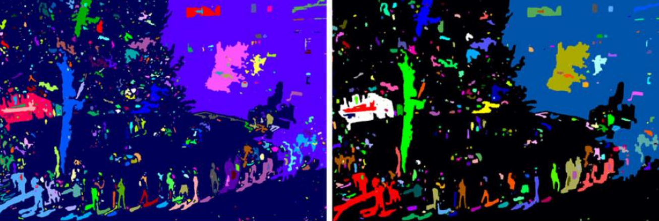
Segmentation involves partitioning an image into distinct regions or objects based on their visual characteristics, such as color, texture, or intensity. This process is essential for various applications, including object recognition, scene understanding, and medical image analysis. By delineating boundaries between different objects or regions within an image, segmentation enables higher-level understanding and interpretation of visual data. Whether it’s identifying individual objects in a scene, separating foreground from background, or isolating specific anatomical structures in medical images, segmentation lays the foundation for advanced computer vision tasks.

Moreover, depending on the different categories that have been chosen, an image can be segmented in more or less detail
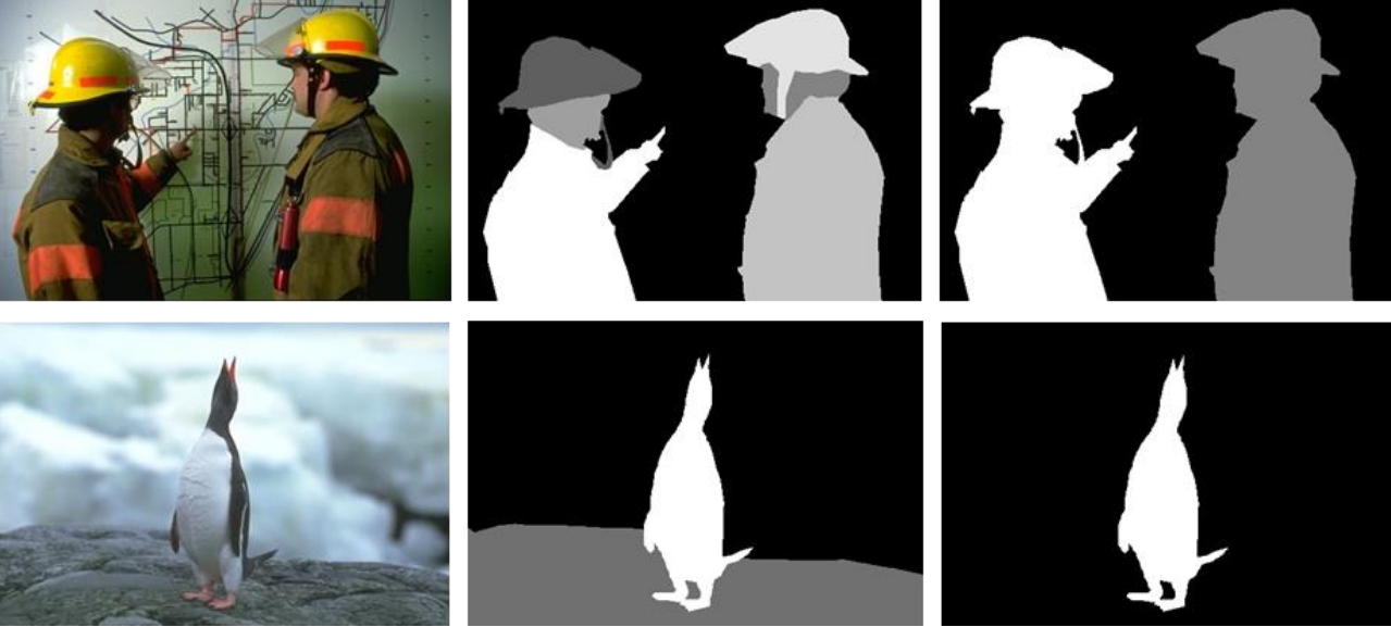
There are two main criteria that can be chosen with respect to the way an image can be segmented. Different parts of the image can be distinguished based on
- Similarity between pixels in the same region
- Discontinuity between pixels in different regions
Such criteria are based on the subdivision of an image into n regions R_1, \, \dots, \, R_n such that
\bigcup_{i=1}^n R_i = R \quad\text{and}\quad R_i \cap R_j = \varnothing \, \forall\,\, i, j \, \text{ st. } (i \neq j)In words: the union of all regions return the original image, and no two regions share space.
We will look into the following techniques:
- Segmentation by thresholding and Otsu’s method
- Region growing
- Watershed
- Clustering-based methods
- Model-based segmentation
- Edge-based methods
- Graph partitioning methods
- Multi-scale segmentation
Segmentation by thresholding
Segmentation by thresholding operates on the principle of setting thresholds, which define the boundaries between different objects or background within an image. By comparing pixel intensities or color values against predetermined thresholds, segmentation by thresholding effectively separates foreground objects from the background. Despite its simplicity, segmentation by thresholding remains a versatile and efficient tool in the computer vision toolkit, offering a quick and intuitive means to extract relevant information from visual data.
Such thresholds may be defined on the histogram. For example, if we were to have the following histogram

It would be very easy to figure out where to put the threshold.
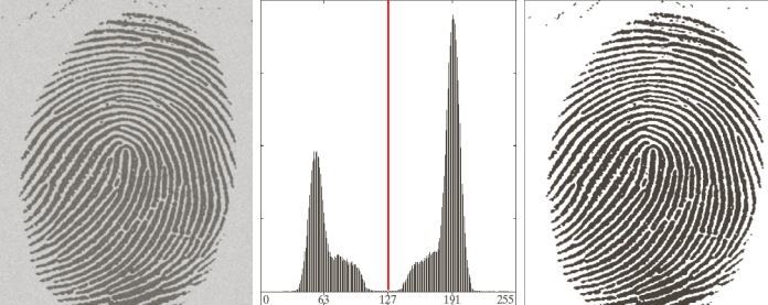
Problems arise when there is noise in the images and the histogram is not as clearly separated anymore.

Or similar things happen when there are changes in the illumination

In other circumstances, the histogram can still be hard to threshold, for example in the case of small regions.

Choosing a threshold can therefore become a very complex task. There is in fact an algorithm that can find the optimal threshold in any circumstance.
Otsu’s optimal thresholding method
Otsu’s technique assumes that two classes are created by thresholding by maximizing the inter-class variance and minimizing the intra-class variance accordingly.
First of all, the normalized histogram must be computed. Once done, we can set a threshold T(k)=k which divides the image in two classes: below threshold P_1 and above threshold P_2. At this point we can compute the probability of a level belonging to the below threshold (which leaves us with the probability of it belonging to the above threshold as well).
Mathematically, we have
P_1(k) = \sum_{i=0}^k p_i\quad\text{with } k = 0, \, 1, \, \dots, \, L-1\\[10pt]

P_2(k) = 1-P_1(k)
We can now calculate the average intensity m_g of the whole image
m_g = \sum_{i=0}^{L-1} i\cdot p_iAnd compute the cumulative mean up to level k
m(k) = \sum_{i=0}^k i \cdot p_iAt this point we can compute the average values of the pixels in the two different classes for all the different values of k \in [0, \, L-1]
m_1(k) = \dfrac{1}{P_1(k)} \sum_{i=1}^k i \cdot p_i\\[10pt]

m_2 = \dfrac{1}{P_2(k)} \sum_{i=k+1}^{L-1} i \cdot p_i
The global variance \sigma_G^2 of all the pixels of the image is
\sigma_G^2 = \sum_{i=0}^{L-1} (i-m_G)^2 \cdot p_1While the inter-class variance \sigma_B^2 is
\begin{aligned}
\sigma_B^2(k) &= P_1 \underbrace{(m_1-m_G)^2}_{\text{mean - general image}} + P_2 (m_2 - m_G)^2\\[20pt]

&=P_1 P_2(m_1-m_2)^2\\[5pt]

&= \dfrac{(m_g P_1 - m)^2}{P_1(1-P_1)} \quad \text{with } k \in [0, \, L-1]
\end{aligned}Note: P_1 and P_2 are functions of k and can be manipulated to obtain the last result.
The quality of the threshold is then defined as
\eta = \dfrac{\sigma_B^2(k)}{\sigma_G^2}The optimal threshold is then found by maximizing \eta, which in turn means finding
k^* \text{ st. } \sigma_B^2(k^2) = \max(\sigma_B^2(k))And we can therefore segment the image using k^* as the threshold.
The intra-class variance and global variance are respectively defined as
\sigma_{\text{in}}^2 = P_1 \sigma_1^2 + P_2 \sigma_2^2\\[5pt]

\sigma_G^2 = \sigma_{\text{in}}^2 + \sigma_B^2
For example, by considering the image on the left, we can obtain the two variances on the right
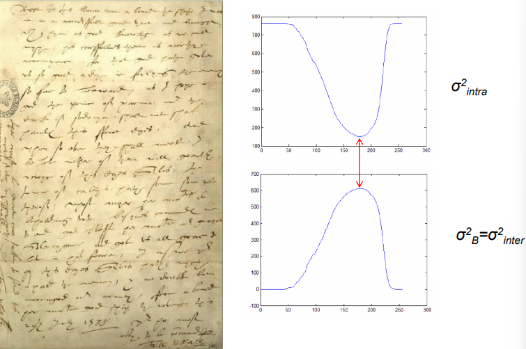
Which when the image gets threshold using them, generates

Otsu’s method works better than other, for example better than the k-means algorithm
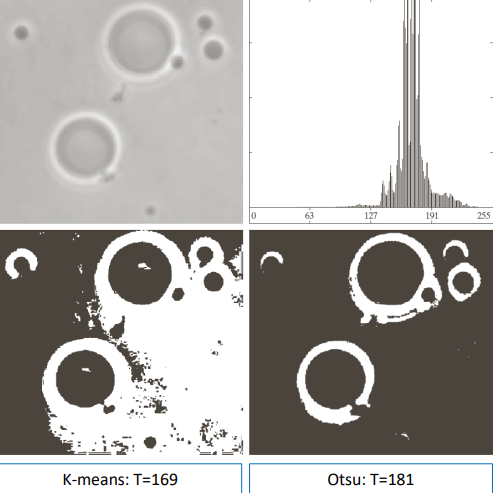
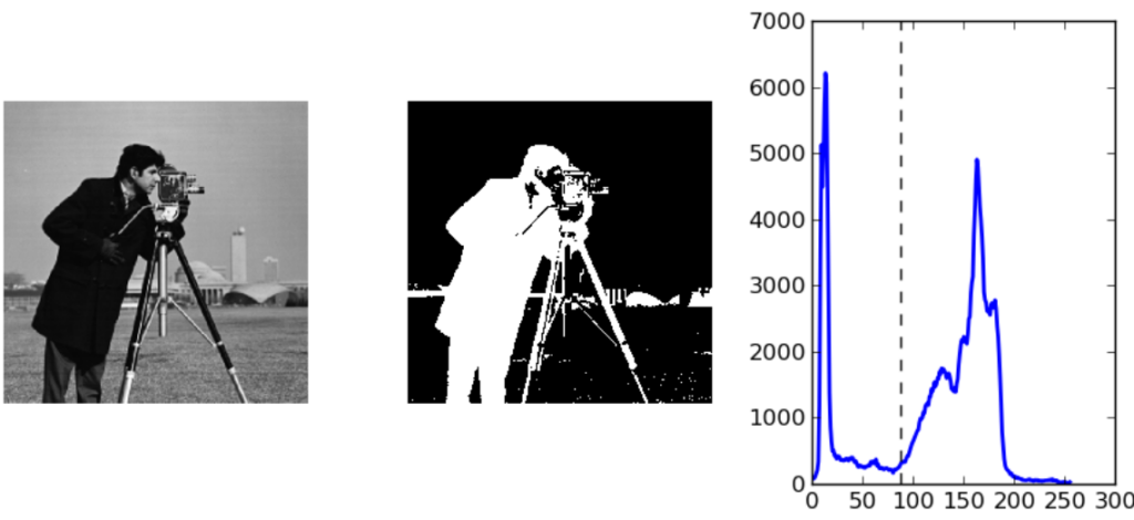
And is able to segment decently complex images
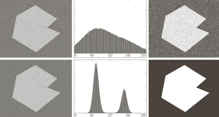
By applying Otsu’s method to images with noise the results are pretty good.
Otsu’s method it’s not perfect though: considering the images below we can in fact see that it’s not always able to threshold images correctly—especially in the presence of smoothing.

Otsu’s method can therefore be combined with other techniques such as edge detection for better results. Generalizations of the same algorithm can be used to find multiple categories in the image, as well as non global thresholding.
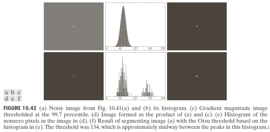
Detecting edges with Otsu
To detect the edges of an image, multiple steps before the application of Otsu can be done to better the results
Multiple thresholds (categories)
By subdividing the image into multiple regions we can still maximize the inter class variance and threshold the image into N total regions (in case N=2 we fall back in the previous analyzed cases).

Non global thresholding
By processing different regions of the image using different thresholds we can apply Otsu’s method to each sub-image individually and then aggregate the results.
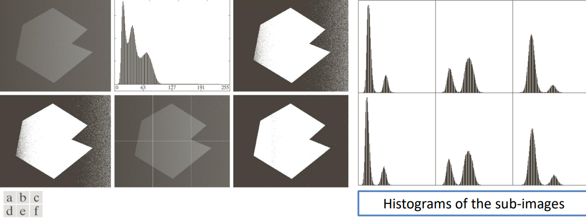
Note: we haven’t covered how the different sub-images have been crated.
Region growing
Region growing provides a powerful method for segmenting images by iteratively grouping pixels into regions based on predefined similarity criteria. This approach starts with seed points or small regions and gradually expands them by incorporating neighboring pixels that meet specified similarity conditions, such as intensity or texture. Through this iterative process, region growing effectively partitions an image into coherent regions.
The starting point of the algorithm are the so called seed points, which satisfy a rule to be defined. we also need a stopping rule and a predicate to control the growing.
Starting from an image f(x, \, y) and a seed array S(x, \, y) of the same size that contains 1‘s (true) at the location of seed points and 0‘s (false) elsewhere. The task is to find connected components in S(x, \, y) and erode each component until one pixel is left.
Once done, we can create a new image f_Q such that
f_Q(x_i, \, y_i) =
\begin{cases}
1 &\text{iff } Q(x_i, \, y_1) \text{ is true}\\
0 &\text{iff } Q(x_i, \, y_1) \text{ is false}
\end{cases}
We can create an image f_G by appending to each seed point in S the 1s if f_Q that are 8-connected to that seed point. 8-connectedness implies that two pixels are connected if they share an edge or a corner (there are four edges and four corners). So, for each seed point in S, f_G will be set to 1 if they are 8-connected to that seed point in f_Q, and 0 otherwise.
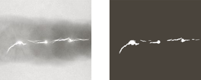
For example, we can consider an x-ray image of welding and our goal is to define which areas have defects. We know that in the case of welding the defects appear as brighter areas in the picture, so we can threshold the image to select only the brightest areas (middle picture). In this case, we selected areas that have a higher brightness than 99.9% of the other areas. We then erode each component until one point is left.

We can now specify a predicate to grow the so found seeds. For example, in this case se can set a threshold such as
Q(x_i, \, y_i) \text{ is true} \iff |f(x_i, \, y_i)-f(x_s, \, y_s)| \leq TAs a final image, after keeping only the values that satisfy the threshold, is
Watershed
The term watershed originates from the field of geography, where it was used to delineate boundaries between drainage basins, the watershed algorithm has found extensive application in digital image processing. In the context of computer vision, the watershed algorithm treats an image as a topographic surface, where pixel intensities represent elevations. By simulating the flooding of this surface from various seed points, the algorithm delineates regions of interest based on the topology of the image, effectively partitioning it into distinct catchment basins. This approach is particularly valuable in segmenting complex images with irregular shapes, such as those encountered in medical imaging, object recognition, and scene analysis. Moreover, the watershed algorithm’s ability to preserve object boundaries makes it a versatile tool for tasks ranging from image segmentation to object counting and tracking, offering significant utility across diverse applications in computer vision and image manipulation.
With this algorithm we can find segmentation boundaries and connected components. The flooding of the surface starts from the point(s) of local minima in the image. When the water level rises, before two basins merge together we can “build a dam” between them: such lines are the boundaries of the segments.
The morphological interpretation of this technique can be seen as a set of subsequent dilations, and the dams are created when dilation merges two components

The same watershed algorithm can be applied on images generated using the gradient. The goal is to extract uniform regions. Gradients are the areas in an image where the intensity changes rapidly, and these areas often correspond to the edges of objects in the image. The watershed algorithm can be used to segment images based on these gradients, by flooding the valleys between the edges until they meet. The watershed algorithm is useful when dealing with small gradients (small gradients correspond to thick edges) because small gradients mean that there is a less pronounced difference in intensity between the edges and the surrounding areas. This can make it more difficult to segment the image using other techniques, however, the watershed algorithm can still be used to segment the image by flooding the valleys between the edges, even if they are not very steep.
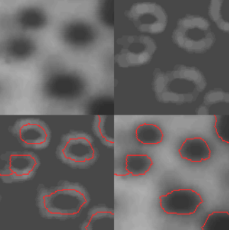
A problem that can arise with this kind of operation is that the final image appears oversegmented due to its noise and irregularities. One possible solution is to define markers which can drive the segmentation with objects of interest. One of the possible ways to define such markers is applying a smoothing preprocessing step
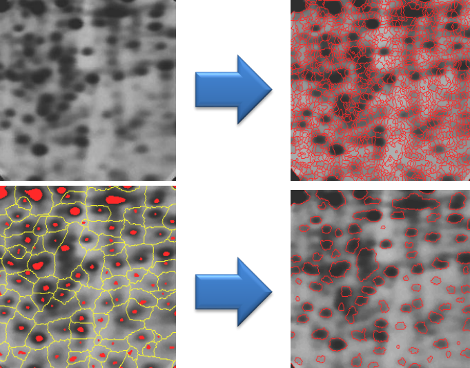
Watershed in OpenCV
OpenCV implements a marker-based watershed algorithm in which the markers are manually selected. The relevant docs can be found here.
Clustering based methods
Clustering-based leverage the inherent structure within image data, clustering algorithms aim to group pixels into meaningful clusters based on their similarity in a feature space. By treating an image as a collection of data points in a high-dimensional space, clustering techniques enable the automatic partitioning of images into coherent regions with similar characteristics. From traditional methods like K-means clustering to more sophisticated techniques such as spectral clustering and Gaussian mixture models, clustering-based approaches play a pivotal role in various computer vision tasks.
For these techniques to work we will represent each pixel with a multi dimensional feature vector. Depending on the task at hand we could include information like the spatial position, the intensity or brightness of the pixel, the color information and many other things. To such characteristics we can apply a suitable clustering algorithm that is able to group pixels based on their vectors by comparing the corresponding features. Thus we need a distance function to compare the vector features. Some common ones that can be used are the following
\text{Absolute value/Manhattan}\\
d_a(\bar{x}_i, \, \bar{x}_j) = \sum_{k=1}^D \lvert x_{i,k}-x_{j,k}\rvert\\[15pt]

\text{Euclidean}\\
d_e(\bar{x}_i, \, \bar{x}_j) = \sqrt{\sum_{k=1}^D(x_{i,k}-x_{j,k})^2}\\[15pt]

\text{Minkowski}\\
d_m(\bar{x}_i, \, \bar{x}_j) = \left[\sum_{k=1}^D(x_{i,k}-x_{j,k})^p\right]^{1/p}
There are two basic approaches to clustering:
- Divisive clustering: this clustering technique starts with a single cluster containing all data points and recursively divides it into smaller clusters. It operates in a top-down manner, iteratively splitting clusters based on dissimilarity measures until each cluster contains only one data point or a predefined stopping criterion is met.
- Agglomerative clustering: this method initially represents each data point its own cluster, which are then iteratively merged based on similarity measures until a termination condition is met.
Another more advanced technique is the k-means algorithm.
K-means clustering
The k-means clustering algorithm operates by partitioning a given dataset into k fixed distinct clusters, where each cluster is represented by its centroid, aiming to minimize the within-cluster sum of squared distances. K-means clustering enables the automatic categorization of pixels into distinct groups based on their feature similarity, facilitating the decomposition of images into semantically meaningful regions. Its simplicity, efficiency, and effectiveness make K-means clustering a widely utilized technique in numerous vision-related tasks, ranging from object recognition and tracking to texture analysis and scene understanding.
Once the process is done, each feature vector is associated with one of the k clusters. Specifically, the k clusters are disjoint sets C_1, \, \dots, \, C_k and we call \mu_j the centroid of the i-th cluster C_i. The objective of the algorithms is to measure the distance between each data point and the centroid of its cluster, whilst minimizing the error made by approximating the points with the center of the cluster it belongs to. Mathematically
\min\left(\sum_{i=0}^k \sum_{x \in C_i} d({\bf x}, \, {\bf\mu_i})\right)\quad\text{where } d(\cdot)\text{ is an appropriate distance}Searching amongst all possible combinations is computationally unfeasible, so we need to define some heuristic that can be used instead.
Lloyd’s algorithm (k-means algorithm)
- We select k centroids. We can choose them according to two methods:
- Forgy method: we randomly select k centroids
- Random partition: we build the k clusters by randomly assigning all the points to some cluster and then computing the centroids
- We associate each point to the closest centroid
C_i = \{ {\bf x} : i = \argmin_j(d({\bf x}), \, \mu_j)\}\quad\text{for }j=1, \, \dots, \, k- We compute the new centroids based on the aggregated points
\mu_j = \dfrac{1}{C_i} \sum_{x\in C_i}{\bf x}- We repeat step 2 and 3 until the centroids do not sensibly move anymore
This algorithms is light and simple, so it is often used for its speed and fast convergence. Optimality is not always guaranteed, though. The solution is dependant upon the initial choice of the centroids and the chosen number of clusters so the best parameters are not necessarily chosen.
Color and intensity clustering
Color and intensity clustering techniques focus on partitioning pixels in an image based on their color or intensity values, respectively. These methods allow the segmentation of images into regions with similar color or intensity characteristics.
For example
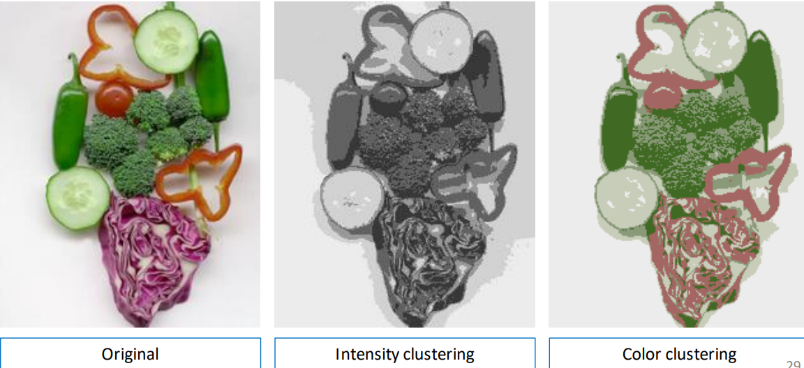
By increasing the number of clusters
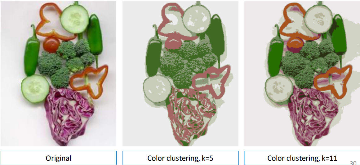
Notes: some of the segments are not connected. Some of the clusters are meaningless and textured objects cannot be segmented properly.
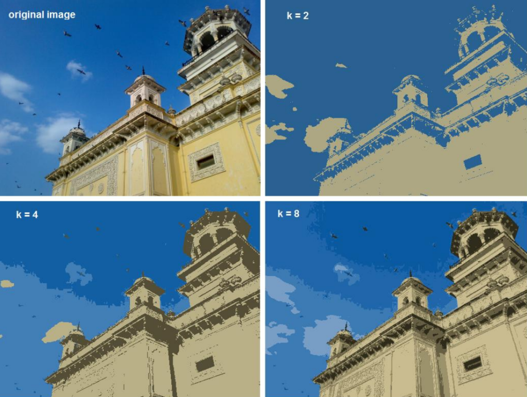
Color clustering
We can also cluster images by using color alone.
Clustering with color and position
If we include the position (spatial coordinates) of each pixel in the feature vector we can split objects that have similar features (and could therefore be in the same cluster), but are in different parts of the image (eg. the cucumber slices).

Model based segmentation
The k-means algorithm is often a good choice for clustering, but it has some problems. One issue is that you need to set the value of k (the number of clusters) before you start. This can be good or bad depending on what you are trying to do, but it doesn’t work well in every situation.
To make k-means better, we can use a density function with “modes” (peaks). When working with images, we deal with pixels, not density functions, so we need to connect the image to its density function somehow.
First, we can pick some sample points. Then, we can use a method called Kernel Density Estimation (KDE), also known as the Parzen window technique. KDE works by combining the sample points with a kernel function to guess the underlying probability density function.
The kernel (such as a Gaussian kernel) has a parameter called bandwidth or radius (denoted by \sigma). This parameter decides the size of the window around each sample point. The kernel function is centered on each sample, and its shape determines how nearby samples affect the estimated density at that point. This process smooths out the discrete sample points, creating a continuous density estimate over the range of values.
After convolution, the result is an estimate of the probability density function. This function provides information about the likelihood of encountering different pixel values within the image.
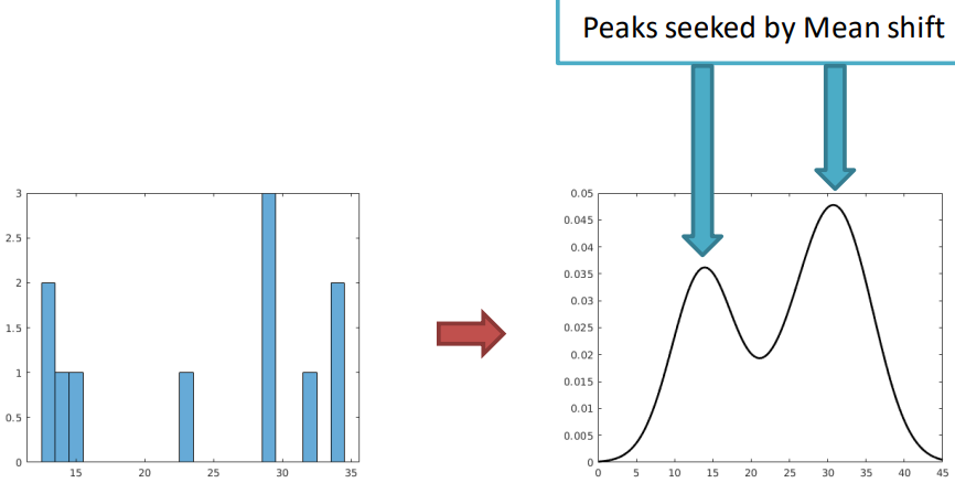
The kernel is defined as
K({\bf x}) = c_k \cdot k\left(\left\|\dfrac{x}{r}\right\|^2\right) = c_k \cdot k \left(\dfrac{\left\|x^2\right\|^2}{r^2}\right){\bf x} is a vector or points in the n-dimensional feature space, and the kernel K(\cdot) integrates to 1 whilst having radius r. The function k(\cdot) (lowercase k) is a 1-dimensional profile that generates the kernel, namely the shape of the kernel function along a single dimension. This profile determines how the kernel function distributes weight or contributes to the estimation of the density at a given point.
The choice of the kernel can be made amongst different shapes, for example
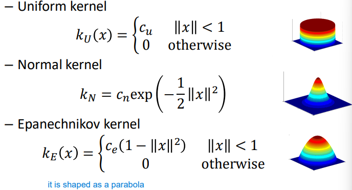
The convolution with a given kernel of radius r is expressed via summation by translating the kernel for each data point. If we were to have N total data points, the convolution would be the result of
f({\bf x}) = \dfrac{1}{N r^n} \sum_{i=1}^N K({\bf x}-{\bf x}_i) = \dfrac{c_k}{N r^n} \sum_{i=1}^N k\left(\dfrac{\|{\bf x}-{\bf x}_i\|^2}{r^2}\right)Where {\bf x}_i are the input samples, and k(\cdot) is the kernel function’s Parzen window.
Note: the factor r^n normalizes the vector according to its number of dimensions, as {\bf x} \in \R^n.
Now that we have found the density function, we can find its modes (the major peaks) and the regions of the input space that we have to climb to reach the higher peaks. To find such density function we have to search through all the n-dimensional space in a very inefficient way so we are going to look into mean shift, which represents an efficient approach to the estimation of the PDF utilizing the gradient.
Mean shift
The essence of mean shift lies in its ability to iteratively adjust the position of data points in a high-dimensional space towards the mode (peak) of a probability distribution without computing the distribution function explicitly. Basically, through mean shift we can find stationary points, amongst which there are the peaks.
The initial assumption of such technique is that the data points are sampled from an underlying PDF, so by estimating the parameters of a PDF like the following
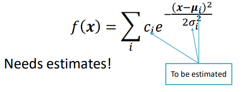
We can get an idea of what the actual function is. For example
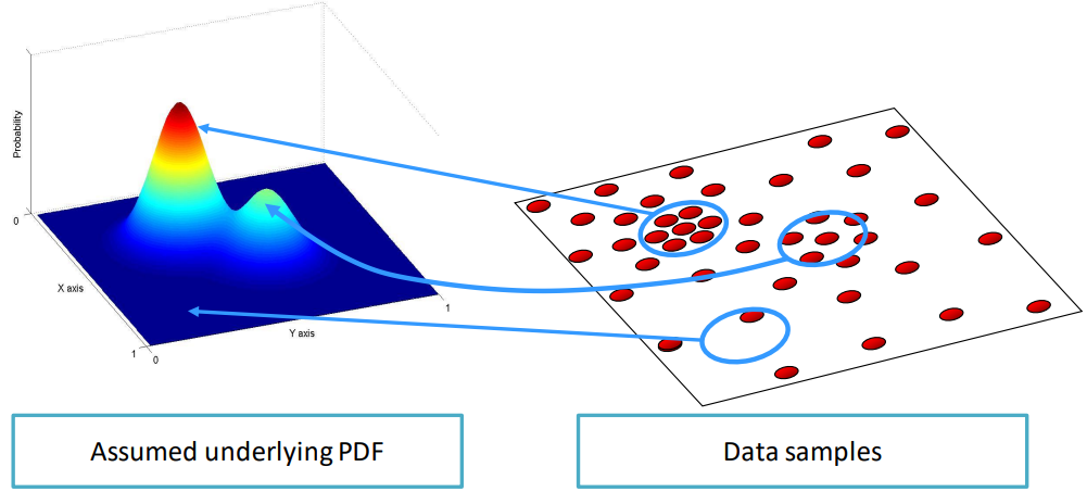
In which the spots in the data point in which there are lots of points correspond to the peaks in the density function, while more sparse points have lower values.
To the same extent, we can use the gradient and perform the so called density gradient estimation, which directly estimates the gradient of the PDF to understand what is the direction of steepest ascent, and therefore the position of the peaks.
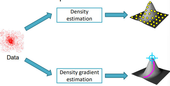
To estimate the gradient we use
\nabla f({\bf x}) = \dfrac{1}{N r^n} \sum_{i=1}^N \nabla K({\bf x}-{\bf x}_i)\quad\text{where } K({\bf x-x}_i)=c_k k\left(\dfrac{\|{\bf x}-{\bf x}_i\|^2}{r^2}\right)Mathematically, the inner gradient of K(\cdot) is the product of c_k k\left(\dfrac{\|{\bf x}-{\bf x}_i\|^2}{r^2}\right) and the derivative of the inner function, which is \dfrac{2}{r^2}\|\underbrace{{\bf x}_i-{\bf x}}_{(\spades)}\|={\bf y}_i. By then calling g(a)=-k(a)=\underbrace{-({\bf x}-{\bf x_i})}_{(\spades)} and grouping all the constant terms, we can express \nabla f({\bf x}) as
\begin{aligned}
\nabla f({\bf x}) &= \dfrac{2c_k}{Nr^{n+2}} \sum_{i=1}^N [({\bf x}_i-{\bf x}) \cdot g({\bf y}_i)]\\

&=\dfrac{2c_k}{Nr^{n+2}}\left(\sum_{i=1}^N [{\bf x}_i \cdot g({\bf y}_i)]-{\bf x}\cdot\sum_{i=1}^N g({\bf y}_i)\right)\\

&=\dfrac{2c_k}{r^2 c_g}\left[\dfrac{c_g}{N r^n}\sum_{i=1}^N g({\bf y}_i)\right]\cdot\left[\dfrac{\displaystyle\sum_{i=1}^N {\bf x}_i \cdot g({\bf y}_i)}{\displaystyle\sum_{i=1}^N g({\bf y}_i)}-{\bf x}\right]
\end{aligned}
Where the constant c_g normalizes the integral in the feature space when g(\cdot) is used as a kernel.
In which each of the terms has the following meaning

Visually, the mean shift vector can be seen as
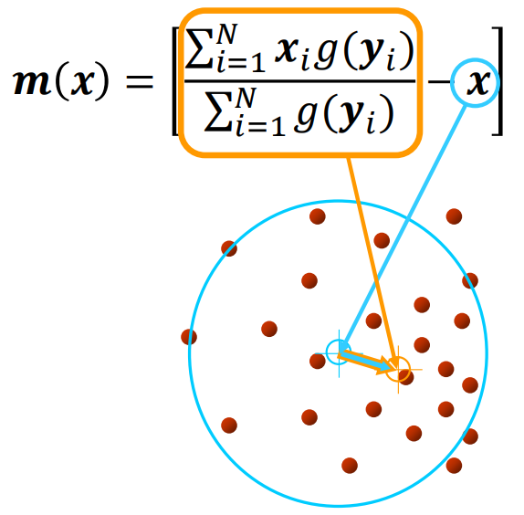
Such vector signifies the direction to follow to find the mode through an iterative procedure:
- We compute the mean shift vector m(x)
- We move the kernel window by m(x)
- We stop when the gradient is close to 0
One last step that must be done to ensure the modes are correctly identified is to prune the mode by perturbation, which allows the saddle points to be discarded. A saddle point in one in which the gradient is 0 but are not peaks, for example
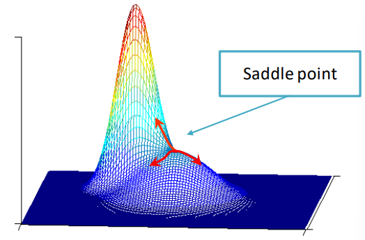
The animation below shows how steps 1 to 3 work in an iterative manner.
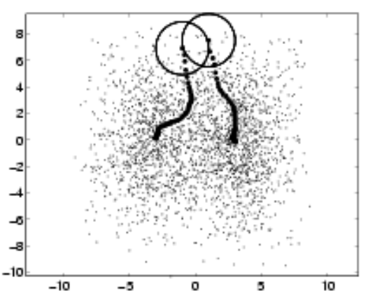
The algorithms stops once an appropriate step size is found after recurrent runs of the algorithm as the vector size gets smaller towards the mode

An optimization that can be done to this algorithm is to divide the space into windows and run the algorithm in parallel on multiple parts of the space

In this case, all the subspaces move towards the same point, but in certain cases, different points might lead to different directions.
Mean shift offers several advantages: firstly, it doesn’t presume clusters to be spherical, allowing it to handle various cluster shapes effectively. Another advantage is its simplicity, as it requires only one parameter, the window size r, making it relatively easy to implement. Moreover, mean shift possesses a physical interpretation, as it converges towards regions of higher density, which aligns with intuitive notions of clustering. It adapts well to datasets with varying densities, thus capable of discovering a variable number of modes. Additionally, mean shift demonstrates robustness against outliers in the data.
However, there are limitations to consider. The performance of mean shift heavily relies on the choice of the window size, which isn’t always straightforward to determine, and an inappropriate selection might lead to mode merging. Furthermore, mean shift can be computationally expensive, particularly for large datasets, and it doesn’t scale efficiently with the dimensionality of the feature space, posing challenges for high-dimensional data analysis.
Mean shift application: clustering and segmentation
Through the use of mean shift we can define the attraction basin as the region for which all trajectories lead to the same mode
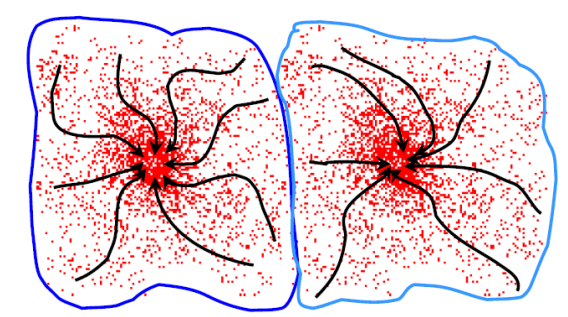
By utilizing such technique we can separate complex modal structures
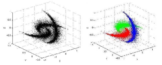
mean shift clustering operates by iteratively shifting data points towards high-density regions, effectively delineating distinct objects or regions within an image. This process is particularly advantageous as it doesn’t necessitate prior assumptions about the number or shape of the clusters, making it well-suited for scenarios with complex or irregularly shaped objects.
Moreover, by using different kernels, through mean shift we can preserve discontinuities by using a joint domain of spatial and color coordinates
K(x) = c_k \cdot k_s\left(\dfrac{{\bf x}_s}{r_s}\right) \cdot k_r\left(\dfrac{{\bf x}_r}{r_r}\right)In which {\bf x}_s are the spatial coordinates and {\bf x}_r are the color coordinates. In the image below, different values for the color window and space window are used
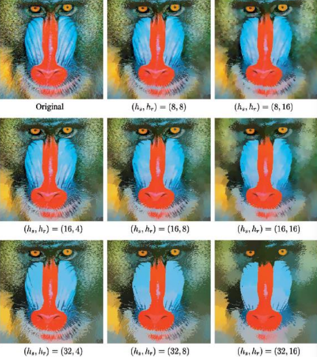
Changing those values change the amount of cartoonish look of the image, while preserving at all times the discontinuities. A clearer picture of how discontinuities are kept is shown below, especially in the area with the grass and tripod

Likewise in the image below
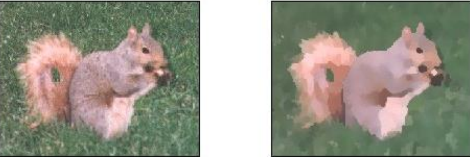
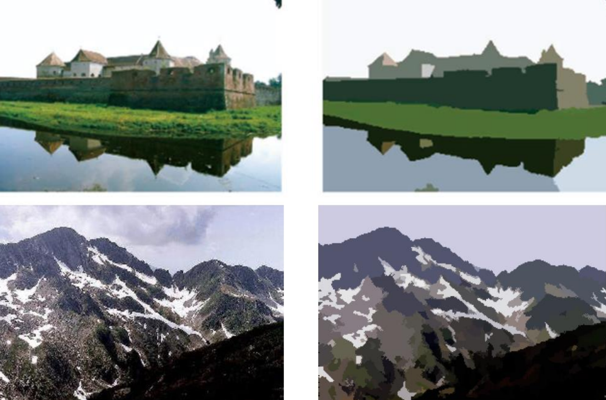
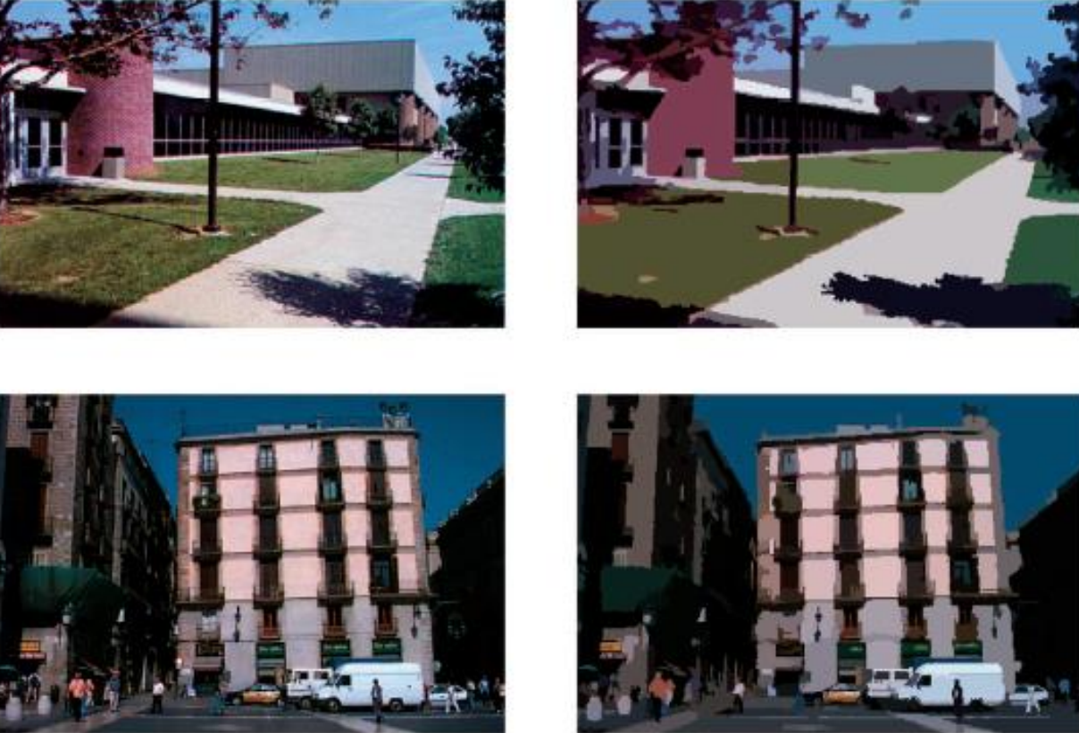
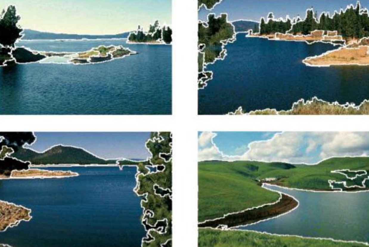
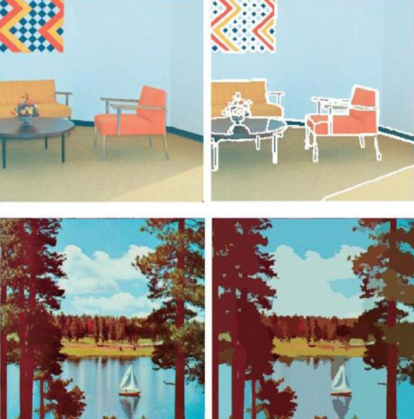
By using the property of preserving discontinuities, we can use the same technique to segment images.
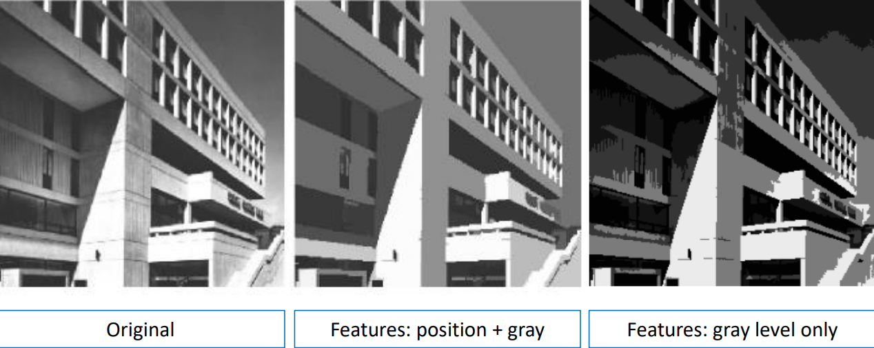
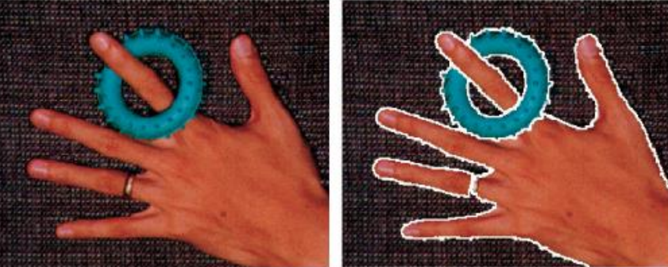
Other examples are shown below.
Markov Random Fields (MRFs)
Markov Random Fields (MRFs) stand as a foundational framework for modeling the complex relationships and dependencies among pixels in an image. Originally rooted in statistical physics, MRFs have become indispensable tools for addressing various challenges such as image segmentation, denoising, and stereo matching. At its core, an MRF represents an image as a graph, where nodes correspond to pixels or regions, and edges encode the pairwise interactions between them.
In this case, segmentation is seen as a per-pixel task, in which each of the pixels (we’ll call the pixel locations sites, and the set of all pixels is called \Omega) gets assigned a label according to an energy function, which we’ll define later. The set of possible labels can be seen as
L=\{\ell_1, \, \ell_2, \, \dots, \, \ell_m\}With |L|=m. In this case we have defined a non-continuous set, but we could also define a continuous one.
Given a pixel location p, its label h is assigned by means of h=f_p=f(p). This labelling is made by using the energy function we mentioned above, composed of two terms: a data term E_{\text{data}}(p, \, f_p) that depends on the specific image features at the pixel location, evaluating how good f_p fits on pixel location p and a smoothing/continuity/neighborhood term \displaystyle\sum_{q\in A(p)}E_{\text{smooth}}(f_p, \, f_q) that depends on the labels in the neighboring pixels—commonly four neighbors are considered. This way, neighboring pixels favour the same label as the adjacent pixels.
The function must be then evaluated over all the pixels in the image, therefore we get
E(f) = \sum_{p\in\Omega}\left[E_{\text{data}}(p, \, f_p)+\displaystyle\sum_{q\in A(p)}E_{\text{smooth}}(f_p, \, f_q)\right]Note: the balance between the two terms is crucial: strong boundaries should be in fact detected without being penalized too much by the smoothing term, as well as the weak boundaries should not affect labeling, as a smoothing term that is too weak could lead to fragmentation.
This model is called Markov Random Field and interactions between pixels are modeled considering a graph in which the connections represent the links of bi-directional mutual influence.
The goal of the MRF is to find the labels that minimize the energy function.
Example 1: random initial seeds for the data term play a crucial role in initializing the MRF. To start the process, one approach involves selecting m random pixels from the image, with each pixel serving as a seed for a specific label or class. These seeds represent initial guesses or references for the different feature classes present in the image.
After selecting the random seeds, the next step typically involves calculating statistics such as the mean and standard deviation within a neighborhood around each seed pixel. This neighborhood defines the local context for computing feature descriptors. For each seed pixel, a feature vector
{\bf x}_i = [I_i, \, \mu_i, \, \sigma_i]^T\quad i \in [1, \, m]is created, where I_i represents the intensity or color value at the seed pixel, while \mu_i and \sigma_i denote the mean and standard deviation of the intensity values within the neighborhood surrounding the seed.
These feature vectors serve as seeds for m different feature classes, with each seed representing a reference point for its respective class. The MRF then utilizes these initial seeds and their associated feature vectors as a starting point for the subsequent optimization process, which typically involves iteratively updating label assignments based on local and global interactions between neighboring pixels, while simultaneously minimizing the energy function defined by the MRF.
After initializing the seeds and feature vectors, the next step involves evaluating the data term, which quantifies the agreement between the observed pixel values and the reference values for each class. One common approach is to use the L_2-norm between the feature vectors of the actual pixel and the reference feature vector of the corresponding class.
Mathematically, this computation corresponds to
E_{\text{data}}(p, \, \ell_i) = \|{\bf x}_i - {\bf x}_p \|_2^2 = \sum_{k=1}^n (x_{i, \, k}- x_{p, \, k})^2Note: n is the feature vector length.
Alternatively, other distance metrics such as the L_1-norm (Manhattan distance) could be employed.
The smoothness term can instead be used to encourages spatial coherence in the labeling of neighboring pixels and any discontinuity in label assignments between neighboring pixels incurs a constant penalty. This penalty term ensures that neighboring pixels with different labels are discouraged, promoting spatially smooth labels.
Mathematically, the smoothness term between two adjacent pixels \ell and h is defined as:
E_{\text{smooth}}(\ell-h)=E_{\text{smooth}}(a) =
\begin{cases}
0&\text{if }a=0\\
c&\text{otherwise}
\end{cases}
c is a constant representing the penalty imposed for label discontinuities.
Example 2: in this case, the data term focuses on identifying peaks in the feature space, representing distinctive characteristics within the image. Initially, m local peaks are selected from the feature space, which serve as reference points for different feature classes. The challenge lies in finding these peaks efficiently, which can be accomplished using techniques such as mean shift clustering.
Once the local peaks are identified, the next step involves associating each pixel with the closest peak. This association process results in finding the corresponding local peaks for each pixel, with the possibility that fewer than m peaks may be found due to the clustering nature.
Regarding the smoothness term, a linear smoothness cost is employed, where the penalty for label discontinuities depends on the distance between labels. The energy associated with a label a relative to a neighboring label b is calculated as
E_{\text{smooth}}(\ell-h)=E_{\text{smooth}}(a)=b\cdot|a|Where b is the cost increase rate. This formulation implies that the penalty increases linearly with the label distance, encouraging neighboring pixels to have similar labels.
A truncated version of this smoothness term is also available, which implies that the smoothness cost is capped at a certain maximum value. This truncation prevents excessively large penalties, providing a more balanced influence between the data term (capturing distinct features) and the smoothness term (promoting label coherence).
Solving the MRF: Belief Propagation (BF)
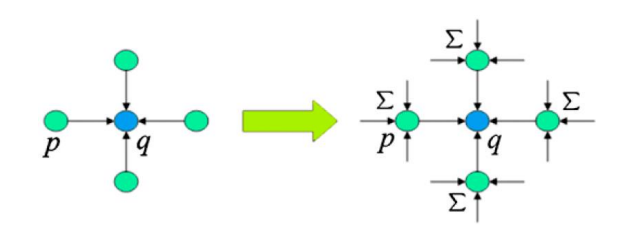
To solve the MRF equation we can use the Belief Propagation technique, which states that neighbouring pixels have information passing through them in the form of a message, which convey information about labels and related costs.
Let’s consider the scenario in which the message sent by pixel p to pixel q contains the local information of pixel p and at the same time the information provided by p’s neighbors in previous iterations. This way, at each iteration of the algorithm, every p in q’s neighborhood passes its message to q, so we get a chain of messages that is being passed on every iteration between pixels
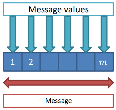
The actual encoding of the message can be mathematically seen as a function that maps the discrete set of labels L into an array of length m having for each position the message value
m_{p\to q}^t(\ell)In words: a message value for label \ell is sent from p to q at time t as a function of the set of labels L.
The actual analytical formulation is

In words: node q inquires all its neighbors, such as p, asking their opinion about selecting label \ell for q. Node p gets the question: to reply, it scans all possible h and tells q about the lowest possible cost then q gets assigned \ell. The reply of node p depends on the data term at p and its smoothing term, as well as the information brought by the neighbors of p at time t-1. The total cost at q is therefore gotten by summing up all the terms in the above equation.
The steps of the BP algorithm are detailed as follows:
- Initialization: at the start of the algorithm, each node in the graphical model initializes its belief state. These beliefs represent the node’s current estimate of the probability distribution over its possible states. Typically, these initial beliefs can be set uniformly or based on some prior knowledge or observations. The equation for the message initialization at time 0 is
m_{p \to q}^0 = \min_{h \in L} (E_{\text{data}}(p, \, h) + E_{\text{smooth}}(h-\ell))While the related costs are
E_{\text{data}}(q, \, \ell) + \sum_{p \in A(a)} m_{p\to q}^0(\ell)- Time update (message passing): the main step of the BP algorithm involves iteratively passing messages between neighboring nodes in the graphical model. These messages contain information about the probability distribution over states that each node sends to its neighboring nodes. At each iteration, a node computes outgoing messages to its neighboring nodes based on incoming messages it receives from other neighboring nodes. This message passing process continues for a predefined number of iterations or until a convergence criterion is met—even though convergence itself might not have been reached. The equations that describe these steps are the ones seen above in the more in depth explanation.
- Termination: the BP algorithm terminates when a stopping criterion is satisfied. This criterion could be a maximum number of iterations reached. The final label at each pixel location is determined as
j = \argmin_{1 \, \leq \, i \, \leq m}\left(c_i^{t_0}\right)BP applications: segmentation
The BP algorithm can be used to segment images by using the labeling criteria to define one or more regions. Segmentation by BP is often applied at multiple resolutions to overlay the results.

