overview:

Introduction to features
Let’s consider the following two images


We can clearly see that the same subject is depicted, even though the two pictures have very different characteristics, both in the perspective on the character as well as in the colors. We need a process to automate the process of recognizing similar characteristics in different subjects.
To this extent, we’ll use what are known as features. Features can be described as a meaningful part of the image, made out of two different components: the detectability (finding an easily detectable point in the image) and the description (what happens in the surrounding pixels around the feature). Visually, the extraction of features produces a set of points together with the description of the region.

All identified keypoints should therefore be:
- Stable and repeatable: their stability is measured by means of repeatability score on a pair of images computed as the ration between the number of point-to-point correspondences that can be established and the minimum number of keypoints of the two images.

- Invariant to transformations (eg. rotations)
- Insensitive to illumination changes
- Accurate
To extract such keypoints, we can utilize the concept of a descriptor. Descriptors encapsulate distinctive attributes or patterns within an image and are typically derived from local image patches or keypoints, capturing discriminative information about their appearance, texture, or shape. Common characteristics of descriptors include invariance to transformations such as rotation, scale, and illumination changes, as well as robustness to noise and occlusions, as well as blur and compression. By encoding salient features of the visual content, descriptors provide a compact and discriminative representation that forms the basis for subsequent processing and analysis in computer vision systems.

Application of feature extraction an matching
Several computer vision systems are based on the features that are contained within images. Amongst the various tasks for which features can be used there are the ones reported below.

Other examples of feature matching are


Or feature tracking
Detecting corners

To find points that are easily recognizable in an image, we can look into corner points.

Those points are in fact the only ones that can yield good results in situations like this one

One way to identify those points is by using the Harris corner detector.
Harris corner detector
By analyzing local intensity variations in different directions, the Harris corner detector excels in its ability to robustly identify key landmarks regardless of scale, rotation, or illumination changes.
Let’s consider a patch in a given position (x_i, \, y_i) and a displacement (\Delta x, \, \Delta y). When we move such patch we can measure how much the content under the moved patch correlates with the content under the patch in its original position. This operation is called autocorrelation, which can be mathematically described as
\tag{$\spades$}E(\Delta x, \, \Delta y) = \sum_i w(x_i, \, y_i)[I(x_i+\Delta x, \, y_i+\Delta y) - I(x_i, \, y_i)]^2In which:
- I is the image
- (\Delta x, \, \Delta y) are the displacements
- i goes over all pixels in the patch
We can now approximate (\spades) with its Taylor series, specifically
I(x_i+\Delta x, \, y_i+\Delta y) \approx I(x_i, \, y_i) + I_x \Delta x + I_y \Delta y
In which I_x = \dfrac{\partial}{\partial x}I(x_i, \, y_i) and I_y=\dfrac{\partial}{\partial y}I(x_i, \, y_i).
In most situations the weights w(x_i, \, y_i) can be neglected, and by canceling out the terms I(x_i, \, y_i) with opposite signs, we can rewrite (\spades) as
E(\Delta x, \, \Delta y) = \sum_i [I_x \Delta x + I_y \Delta y]^2
Which can be rewritten in matrix form as
E(\Delta x, \, \Delta y) = [\Delta x, \, \Delta y]
\underbrace{
\begin{bmatrix}
\displaystyle\sum I_x^2 & \displaystyle\sum I_x I_y\\[10pt]

\displaystyle\sum I_x I_y & \displaystyle\sum I_y^2
\end{bmatrix}
}_{\text{Auto-correlation matrix}}
\begin{bmatrix}
\Delta x\\
\Delta y
\end{bmatrix}
The auto-correlation matrix A describes how the region changes for a small displacement. Such matrix is real and symmetric, therefore its eigenvectors are orthogonal and point to the directions of maxima data spread. The eigenvalues are instead proportional to the amount of data spread in the direction of the eigenvectors.

Examples of how the eigenvectors and eigenvalues change over different distributions is shown below.

By studying the eigenvalues we get information about the type of patch that is bein considered. Specifically, if both eigenvalues are small we are dealing with a uniform region. If one one of the eigenvalues is large we are dealing with an edge, and if both eigenvalues are large we are dealing with a corner.
If we now wanted to add back the weights we removed earlier we could include them by expressing them as a convolution with the matrix. A would therefore become
A = w*\begin{bmatrix}
\displaystyle\sum I_x^2 & \displaystyle\sum I_x I_y\\[10pt]

\displaystyle\sum I_x I_y & \displaystyle\sum I_y^2
\end{bmatrix}
Those weights usually have either values 1 inside the patch and 0 elsewhere, or they might use a gaussian distribution to give more emphasis on changes around the center and discard the other values with decreasing weights.
Whichever weights are decided, a keypoint is selected using one of the following options presented in the literature:
- Minimum eigenvalues [Shi, Tomasi]
- \det(A)-\alpha\cdot\text{trace}(A)^2 = \lambda_0\lambda_1-\alpha(\lambda_0+\lambda_1)^2 [Harris]
- -\lambda_0 -\alpha \lambda_1 [Triggs]
- -\dfrac{\det(A)}{\text{trace}(A)} = \dfrac{\lambda_0\lambda_1}{\lambda_0+\lambda_1} [Brown, Szeliski, Winder]
Overall, the Harris corner detector exhibits properties that distinguish it. Notably, it showcases invariance to brightness offset, meaning that the addition of a constant value to the intensity of every pixel in an image does not affect its ability to detect corners. Moreover, the detector remains invariant to shifts and rotations, ensuring that corners maintain their distinct shapes even when the image undergoes translation or rotation transformations. However, it’s important to note that the Harris corner detector is not inherently invariant to scaling, implying that changes in the scale of an image may impact its corner detection capabilities.
Example usage of the Harris corner detector are shown below


Other corner detectors: USAN
The Univalue Segment Assimilating Nucleus (USAN) operates by identifying coherent regions within an image based on their intensity and spatial coherence. By assimilating pixels with similar attributes into unified segments, USAN facilitates the extraction of meaningful structures and objects from complex visual data. This approach transcends traditional segmentation methods by leveraging both local and global information, thereby enabling more robust and accurate interpretations of images across diverse applications such as object recognition, scene understanding, and medical imaging.
Practically speaking, USAN compares the central point (nucleus) of the mask with the other pixels in the mask. The USAN represents the portion of window with intensity difference from the nucleus within a given threshold.

Depending on the USAN ratio, we get that

When considering the smallest-USAN we get the SUSAN. SUSAN focuses on detecting the uniform regions or potential points of interest without relying on specific thresholding techniques, making it robust to variations in illumination and noise.
Example usage of USAN are shown below


Blob features
While up till now we have focused on features that are based on specific points, other features focus on blobs. A blob is a region in which the properties are different from the surrounding regions, while being constant inside the region.
Maximally Stable Extremal Regions (MSER) are connected areas that are characterized by almost uniform intensity, surrounded by a contrasting background. The Maximally Stable Extremal Regions (MSER) feature detector can be used as a blob detector. MSERs are areas with almost uniform intensity surrounded by contrasting blobs.

MSER was developed to address challenges such as illumination variations, occlusions, and noise: it offers a principled approach to identifying stable and distinctive regions within an image. By characterizing regions that remain consistent across different scales and thresholds.
In essence, the algorithm operates by sequentially applying thresholds to the grayscale image, generating a series of binary images representing regions of varying intensity. Following this, it computes connected regions within each binary image, forming distinct blobs or segments. For each identified region, the algorithm calculates pertinent statistics such as area, convexity, and circularity, which serve as descriptors of its shape and characteristics. Finally, the algorithm assesses the persistence of each blob across different thresholds, determining its stability and significance in the image.
By using this algorithm we can find multiple thresholds in an image

Using different scale to detect objects
Different objects can be detected when using different scales, trivially, detection at different scales can be seen as zooming out on a map, from which only certain features can be detected.

In the image domain, different scales can be used to obtain a different amount of details in the image. Let’s consider the following image

The house in the image above contains only the “main features” that make it a house, and this can be used to facilitate object detection by creating what are known as image pyramids. Image pyramids are composed of a recursive low pass + high pass analysis of an image, which can increase the ability to identify the correct features in the image.


Signal wise, the original image is transformed into a family or derived signals with a parameter t that controls the location in the scale space
f(x, \, y) \to f(x, \, y, \, t)
This way, fine-scale details are gradually suppressed.

Simplifications in the image now arise, and only the strongest elements remain.
To practically implement this, we’ll use the gaussian smoothing. Specifically, the N-dimensional gaussian kernel defined by g: \R^N \times \R_+ \to \R
\tag{$\spades$}g({\bf x}, \, t) = \dfrac{1}{(2\pi\sigma^2)^{N/2}}\exp\left(\dfrac{-(x_1^2+\cdots+x_N^2)}{2t}\right)The scale space is represented as
L(x, \, t) = \int_{\xi \in \R^N} f(x-\xi) g(\xi, \, t)\, d\xiWhere g(\cdot) is the gaussian kernel defined in (\spades).
Note: the expression for L is very similar to a convolution.
For example, by setting t=0 we consider the base version of an image. Increasing the value of t the images get blurrier and blurrier.


In this process, no new local minima are created, so the main features of the image remain there and can be used to detect edges.

The edge detection algorithm can be run for each value of t and then combine the edges found at multiple scales.
Normalizing the strength of edge responses by t ensures that the measurements are adjusted according to the sensitivity level used for edge detection. By doing so, we achieve consistency in comparing edge strengths across various levels of sensitivity, providing a more reliable assessment of edge prominence in the image.
Strong edges can in fact be found for any value of t, and while for smaller values many spurious edges get detect, for higher ones the detected edges are inaccurate.


By combining the different edges and normalizing them, the detected edges are more refined and accurate.