Object recognition
Object recognition is a general term to describe a collection of related computer vision tasks that involve identifying objects in images or videos.
It differs from image classification as this task involves associating one or more categories to a given image, while mere object recognition could just involve finding the location of the objects of interest without assigning them a category tag.
Object detection/localization involves finding the bounding boxes of the objects within an image.
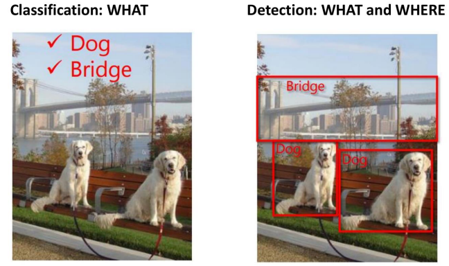
In the case of segmentation, each pixels could be associated with a specific class to find the contours of each object.
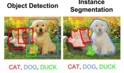
Each object detection task must be able to deal with:
- Different camera positions

- Perspective deformations

- Illumination changes

- Intra-class variance

Template matching
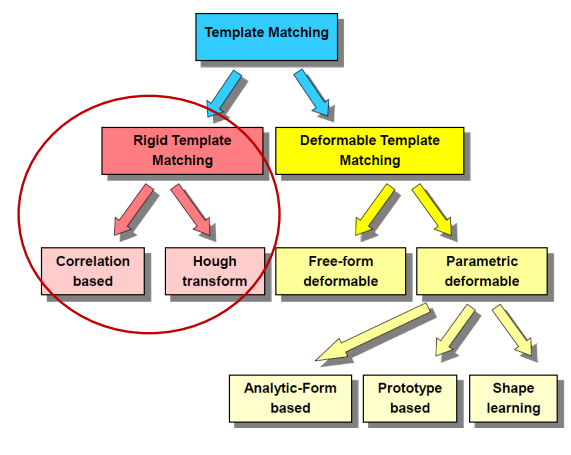
A template is something that can be used as a model to match against other images. The task of template matching is to find instances of the template in the image according to some similarity measure.
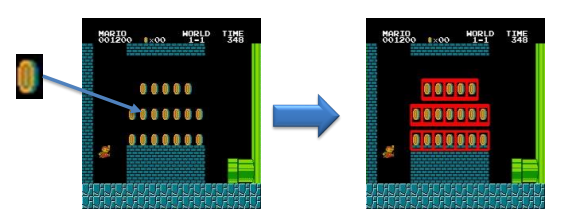
Some of the challenges involved with this technique are the high template variability and the possible deformations that the objects can have, as well as the application of affine transformations or the presence of noise or illumination differences.
Moreover, even simple differencing techniques don’t necessarily provide reliable results.
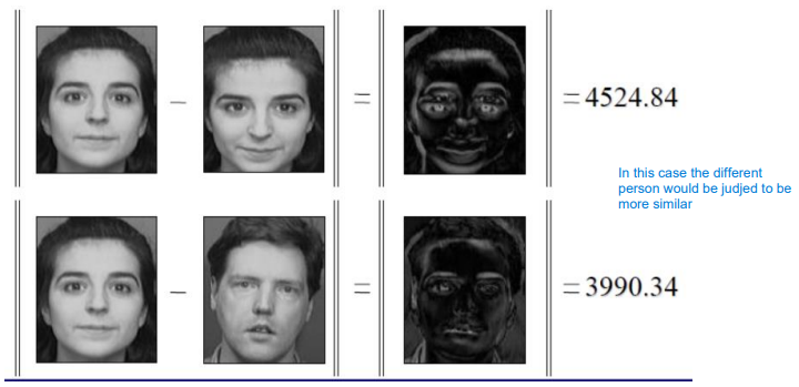
Correlation based
In the context of correlation-based template matching techniques the method used to detect the presence of a certain object involves using a template T that get places in every possible position across the image. This process involves sliding the template over the image, aligning it with different regions, and comparing it to the corresponding parts of the image. We just use the basic approach that doesn’t involve scaling or rotating such templates.
Ultimately, a comparison method is used to determine the similarity between the template and each region of the image. These methods include:
- Sum of Squared Differences (SSD): Measures the squared difference between corresponding pixel values in the template and image region
\phi(x, \, y) = \sum_{u, \, v \, \in \, T} (I(x+u, \, y+v) - T(u, \, v))^2 - Sum of Absolute Differences (SAD): Measures the absolute difference between corresponding pixel values
\phi(x, \, y) = \sum_{u, \, v \, \in \, T} \lvert I(x+u, \, y+v)-T(u, \, v)\rvert - Zero-Normalized Cross-Correlation (ZNCC): Measures the normalized cross-correlation between the template and image region, taking into account variations in brightness and contrast
\phi(x, \, y) = \dfrac{\displaystyle\sum_{u, \, v \, \in \, T}\left(I(x+u, \, y+v) - \bar{I}(x, \, y))\cdot (T(u, \, v)-\overline{T}\right)}{\sigma_I(x, \, y)\cdot \sigma_T}
Note:
- \bar{I}(x, \, y) represents the average on a certain window of the image
- \overline{T} represents the template average
- \sigma_I(x, \, y) is the standard deviation on the image window
- \sigma_T is the standard deviation on the template
Generalized Hough transform
Already seen in a previous section here.
Bag of words (BoW)
The bag of words technique, originally inspired by document analysis, has been adapted and widely utilized in image and object classification tasks. This method is designed to be invariant to various factors, particularly viewpoint changes and deformations, making it robust in diverse scenarios.
At its core, the bag of words technique decomposes complex patterns in images into (semi) independent features, allowing for efficient analysis and classification. Just as in document analysis where words are treated as independent features, in image classification, visual features are extracted from local image regions and aggregated into a “bag of words” representation.
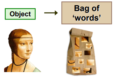
The bag of words technique enables the classification of images based on their content, regardless of specific geometric transformations or distortions.

By searching the dictionary that contains all the features different images can then be matched with them to recognize the content.
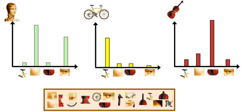
The first step that must be done before doing the matching is the extraction of meaningful keypoints and descriptors
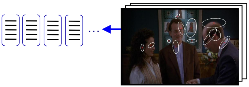
To then be able to cluster those features
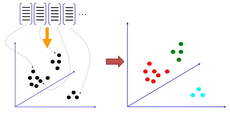
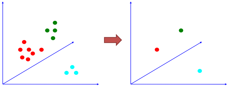
And use each cluster to represent the different classes using a representative sample, for example the centroid.
Convolutional neural networks (CNNs)
When applying deep learning on images, we can treat the image as a 2D matrix
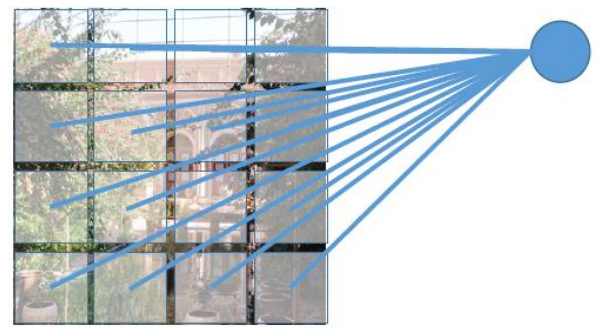
In convolutional neural networks (CNNs), local connectivity refers to the concept that each neuron in a convolutional layer is connected to only a local region, known as its receptive field, in the previous layer. This arrangement allows the network to capture spatial information effectively, as each neuron is responsible for processing a specific region of the input.
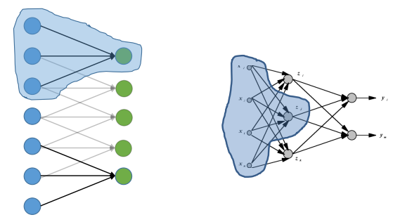
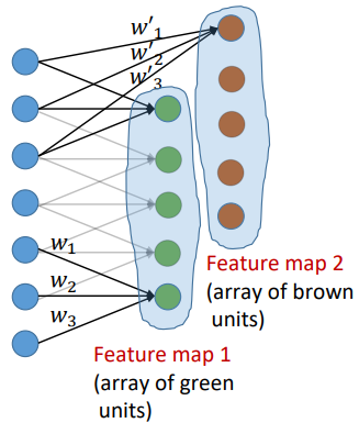
Shared weights further enhance this spatial sensitivity by enforcing weight sharing across the receptive fields of neurons, resulting in spatially invariant responses to certain features. The different weights are combined using convolution operations.

Additionally, CNNs typically employ multiple feature maps in each convolutional layer, enabling the network to learn diverse sets of features from the input data.
Finally, subsampling, often achieved through pooling layers, is used to reduce the dimensionality of feature maps while preserving their essential features.
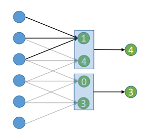
Often, the pooling operations is coupled with a convolution operation to extract meaningful features from the image.
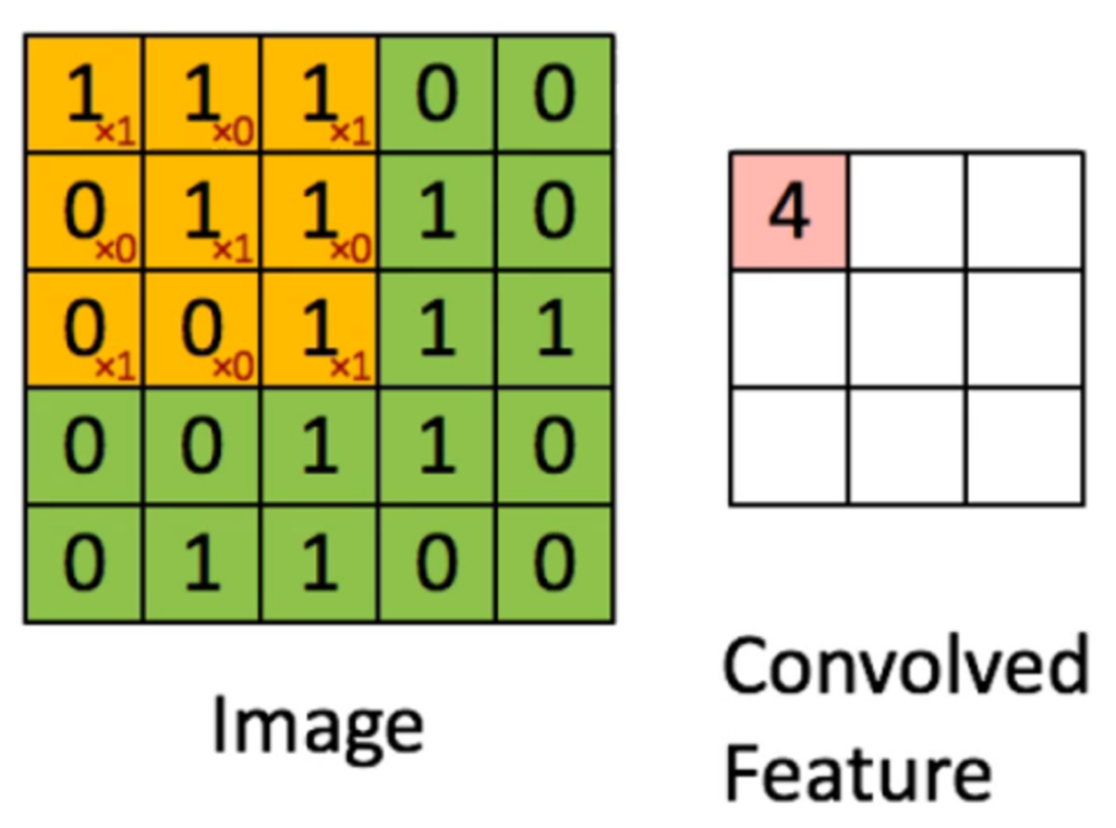
An example is shown below.
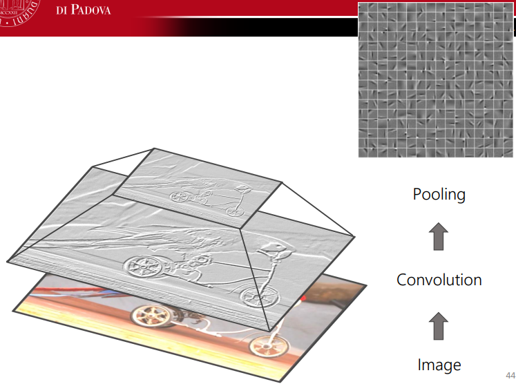
Combining together all the aforesaid steps, we get:

Regularization strategies
Regularization strategies are essential techniques to prevent overfitting and improve the generalization ability of models. Dropout is a widely used regularization method in neural networks, where units are randomly dropped out, or deactivated, during training with a fixed probability p. This encourages the network to learn more robust and distributed representations by preventing co-adaptation of neurons.
L2 weight decay, another common regularization technique, penalizes large weights by adding a regularization term to the loss function proportional to the squared magnitude of the weights. The regularization strength, controlled by an adjustable decay value, determines the degree of penalization for large weights, thereby encouraging simpler models.
Early stopping is a straightforward regularization approach that halts the training process when the performance on a validation dataset fails to improve after a certain number of subsequent epochs, referred to as the patience parameter. By preventing the model from continuing to learn on noisy or irrelevant information, early stopping helps prevent overfitting and results in models that generalize better to unseen data.
Preprocessing strategies
Data augmentation is used to enhance the diversity and variability of training data by introducing variations such as noise, rotation, flipping, and adjustments to hue, color, and saturation. The augmented data enriches the training dataset and helps improve the robustness and generalization ability of models.
Batch processing
The mini-batch gradient descent technique involves using a small batch of data samples for each iteration of the optimizer instead of the entire dataset. This not only accelerates the gradient computation process but also helps alleviate memory constraints by processing only a subset of the data at a time.

