Local operations play a pivotal role in enhancing the efficiency and effectiveness of image processing. These operations focus on specific regions within an image, allowing for targeted analysis and manipulation of pixel values. By honing in on localized features, such as edges, textures, or patterns, local operations empower computer vision systems to extract meaningful information, recognize objects, and make informed decisions. Whether employed for image enhancement, feature extraction, or object detection, the strategic application of local operations contributes to the overall robustness and precision of computer vision algorithms, fostering advancements in fields ranging from automated surveillance to medical imaging. In this context, understanding and harnessing the potential of local operations form a cornerstone in the pursuit of more sophisticated and accurate visual perception systems.
Specifically, on the practical side, local operations consider not only the center pixel that we are working with, but also the neighbouring ones.
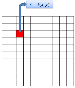

We can now define a kernel using all selected pixels. The choice of a specific kernel allows us to apply different effects on the image, weighting each pixel differently in the final image.
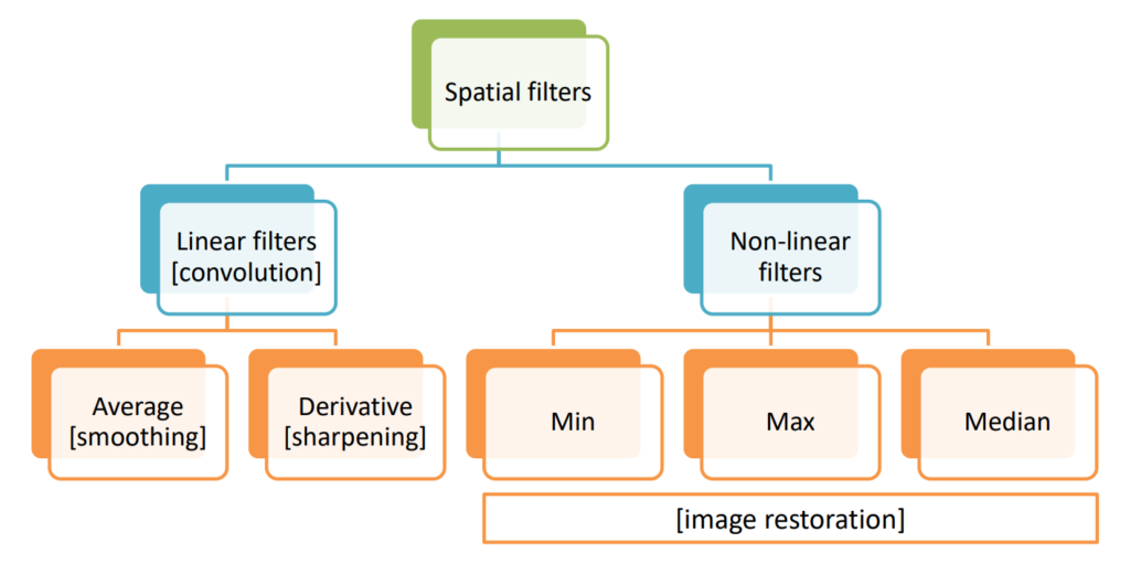
Local operations are therefore performed in the spatial domain of the image. The main operations that can be done are:
- Linear filters (Convolutions / correlations):
- Averaging filters (smoothing)
- Derivative filters (sharpening)
- Non-linear filtering
- Min
- Max
- Median
Correlation / Convolution
Correlation
Correlation acts as a powerful tool for understanding relationships and patterns in visual data. In this context, correlation involves the systematic comparison of pixel values between different regions of an image, enabling the identification of similarities or dissimilarities. Whether utilized for template matching, object recognition, or feature extraction, the application of correlation algorithms provides a mechanism for detecting and interpreting complex visual information.
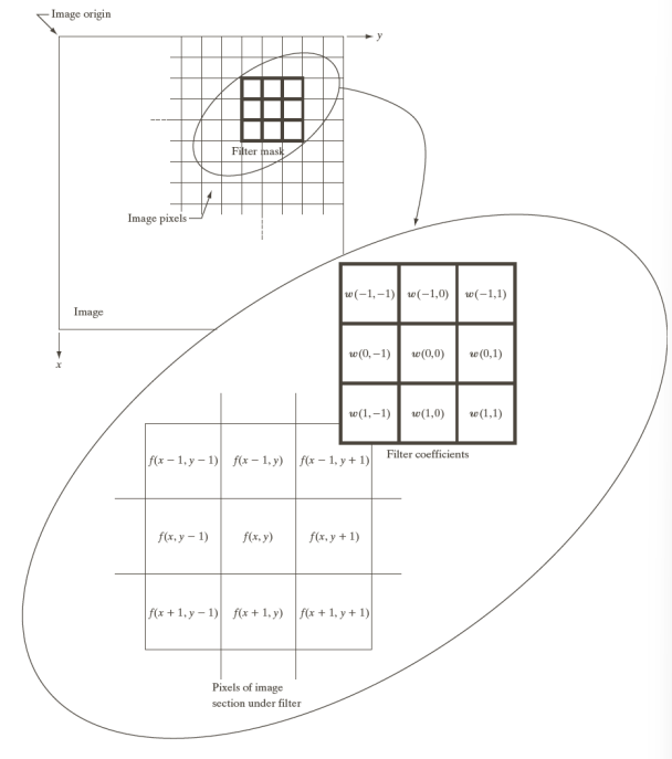
The filter is superimposed on each pixel location of the image, evaluating it by accounting for the pixel value and the filter weight of that specific image.
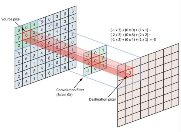
Let’s suppose the filter dimensions are m \times n, we have, where a and b are represent the half-height of the filter and the kernel, respectively
- -m = 2a +1
- -n = 2b+1
Correlation is then defined as
g(x, \, y) = \sum_{s\,=\,-1}^{a} \sum_{t\,=\,-b}^{b} w(s,\, t) I(x+s, \, y+t)Graphically:
Convolution
The convolution of a signal is defined as
(f*g)(t) = \int_{-\infty}^{+\infty} f(\tau) g(t-\tau)\, d\tauWhich has to be quantized into the spatial domain by turning it into a sum
g(x, \, y) = \sum_{s=-a}^{s=a} \sum_{t=-b}^{t=b} w(s,\, t) I(x-s, \, y-t)The correlation that we analyzed above has the following equation
g(x, \, y) = \sum_{s\,=\,-1}^{a} \sum_{t\,=\,-b}^{b} w(s,\, t) I(x+s, \, y+t)In which the only difference are the + and - signs in the I(\cdot) function. In fact, correlation and convolution, despite being mathematically different, when used with symmetric kernels, become equal.
Brightness of an image and filters
The use of filter changes the brightness of the image. Only when
\sum_i w_i = 1
The brightness remains constant.
Averaging filters: smoothing
The kernel for averaging filters is usually one of the following two
\underbrace{
\dfrac{1}{9} \times
\begin{bmatrix}
1&1&1\\
1&1&1\\
1&1&1
\end{bmatrix}
}_{\text{True averaging}}
\qquad

\underbrace{
\dfrac{1}{16} \times
\begin{bmatrix}
1&2&1\\
2&4&2\\
1&2&1
\end{bmatrix}
}_{\text{Another filter widely used}}
The effect obtained is shown below

The images on the bottom are obtained by increasing the size m of the filter.
Instead of applying a matrix filter, if the size of the matrix is n \times n, the filter can be divided into two vector filters of sizes
- n \times 1
- 1 \times n
Computationally, applying a square matrix filter is slower than applying two vector filters one after the other to obtain the same effect. We can therefore separate the filter as
w(x, \, y) \to w_x(x) w_y(y)
The time complexity of the algorithm goes from O(MNab) to O(MN(a+b)).
For example, applying the horizontal and vertical vector filters we get

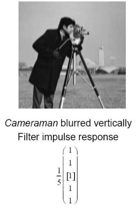
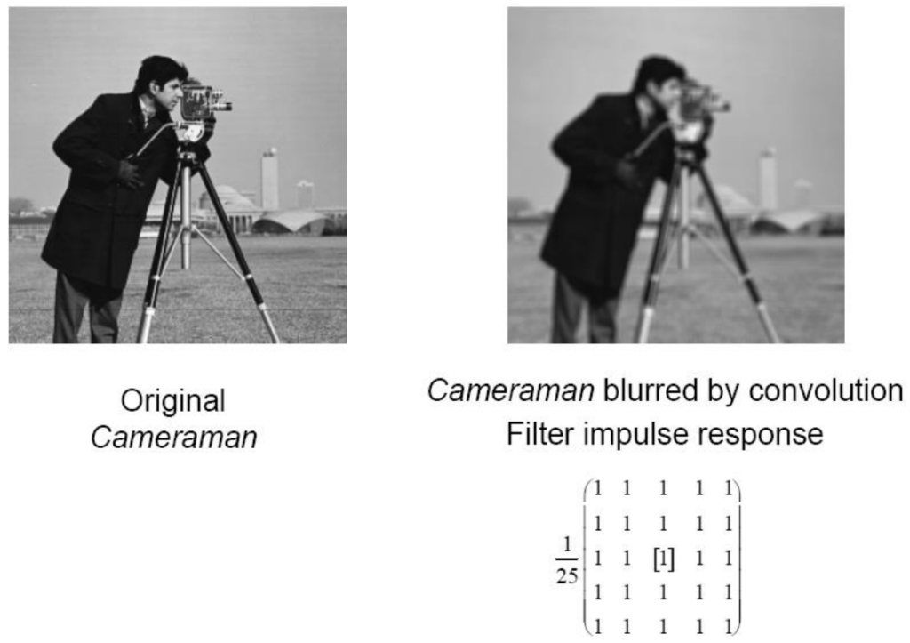
Which is the same effect as applying the matrix filter directly
Derivative filters: sharpening
The derivative operator has the following properties for the first and second order
First order derivative operator:
- Is zero in flat segments
- Is non-zero on the onset of a step/ramp
- Is non-zero along ramps
Second order derivative operator:
- Is zero in clat segments
- Is non-zero on the onset and at the end of a step/ramp
- Is zero along ramps of constant slope
Specifically, looking at the following function (left image)

We can see that (on the right image), both the first and second derivative are always 0 for flat segments. For first order derivatives, the intensity value is given by the change in values between the points n+1 and n. For example, for the first sloped part of the function, for each step in the x direction, the change in intensity if of 1 unit, so the first derivative is constant at -1. For the step instead, the change is 6-1=5, so there is a peak in the first derivative, and then it goes back to 0.
Regarding the second derivative, we can instead observe that is is non-zero only when there is a change in slope at the end and beginning of ramps. Namely, the first point of the intensity transition is calculated by considering (n+1)-n and the final point by considering (n-1)-n.
Mathematically, there are two ways to compute the first derivative:
- \dfrac{\partial f}{\partial x} = f(x+1)-f(x), computed at x+\dfrac{1}{2}
- \dfrac{\partial f}{\partial x}=\dfrac{f(x+1)-f(x-1)}{2}, computed at x but with lower precision
Regarding the second order derivative we can instead write
- \dfrac{\partial^2 f}{\partial x^2} = f(x+1) + f(x-1) - 2f(x), computed at x
The different differential operators that are available for the first order are the following
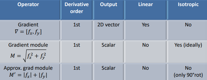
Gradient computation
Derivative operations in computer vision are implemented using filters, which can be applied directly with small kernels or with larger kernels for increased stability and accuracy. The choice between these approaches depends on the specific requirements of the task at hand, considering factors such as computational efficiency, noise robustness, and the desired level of detail in the extracted features.
For example, considering a 3 \times 3 matrix
\begin{bmatrix}
z_1 & z_2 & z_3\\
z_4 & z_5 & z_6\\
z_7 & z_8 & z_9
\end{bmatrix}
In which all the z_i correspond to an intensity value of the image, we can apply the Roberts cross gradient operators
\underbrace{
\begin{bmatrix}
-1&0\\
0&1
\end{bmatrix}
\qquad
\begin{bmatrix}
0&-1\\
1&0
\end{bmatrix}
}_{\text{Robert's operators}}
Or the Sobel operators
\underbrace{
\begin{bmatrix}
-1&-2&-1\\
0&0&0\\
1&2&1
\end{bmatrix}
}_{\dfrac{\partial f}{\partial y}}
\qquad
\underbrace{
\begin{bmatrix}
-1&0&1\\
-2&0&2\\
-1&0&1
\end{bmatrix}
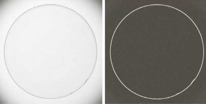
}_{\dfrac{\partial f}{\partial x}}Note: with derivative filters all matrices sum up to zero, which in turn makes the final image darker.
Applying the Sobel filter to the left image, we in fact get the image on the right
Second order derivatives

The Laplacian filter implements the equation
\begin{aligned}
\nabla^2 f(x, \, y) &= \dfrac{\partial^2 f}{\partial x^2} + \dfrac{\partial^2 f}{\partial y^2}\\
&= f(x+1,\, y) + f(x-1, \, y) + f(x, \, y+1) + f(x, \, y-1) -4f(x, \, y)
\end{aligned}
Using that equation, we can construct the following filter. In the two matrices below the only difference are are the signs, often found in practical applications
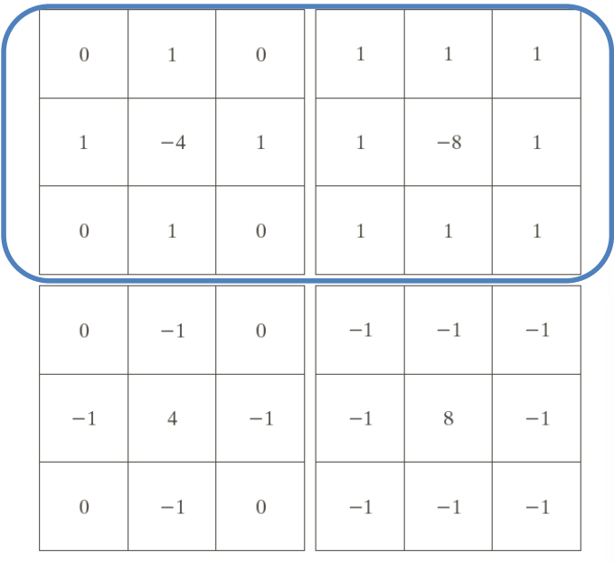
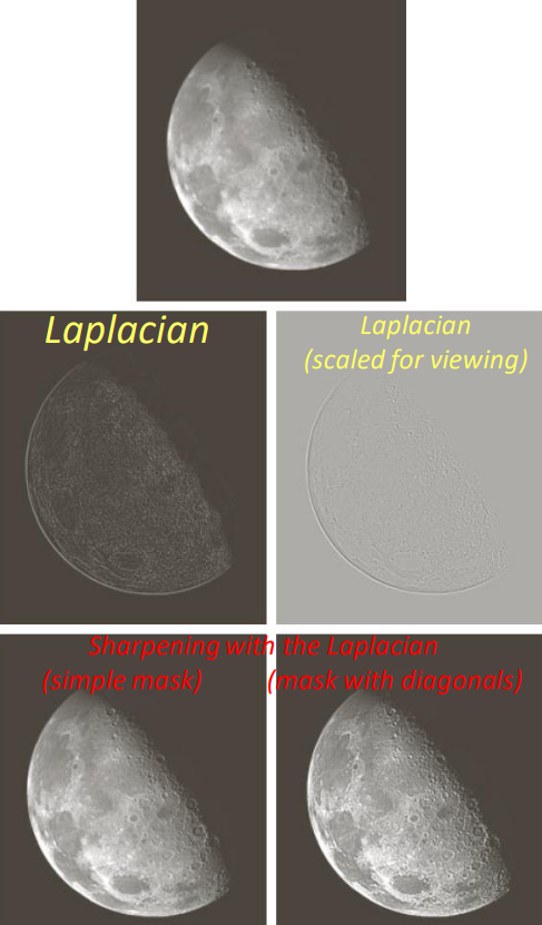
Laplacian filters can be used to enhance the transitions in an image. In practical applications, the Laplacian can be used to sharpen an image, subtracting it if the center weight is negative, or adding it if it’s positive. In case of negative center weights (first 2 matrices), the formula is
g(x, \, y) = f(x, \, y) - \nabla^2 f(x, \, y)
Which results in the following modified images
Other examples of the sharpening by Laplacian filters can be seen in image c below (* represents the product between c and e, not convolution).
Image a is the original scan. Interesting comparisons are g and h with a.
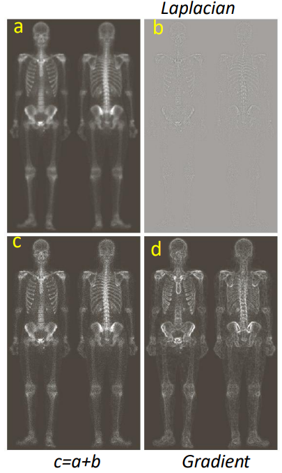
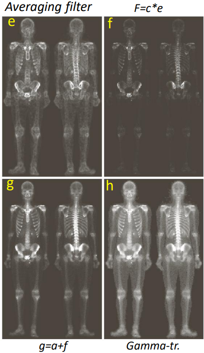
Image restoration
By mowing towards image restoration we are now going to analyse the non-linear filters:
- Min
- Max
- Median
In general terms, image restoration focuses on enhancing the quality of digital images degraded by various factors such as noise, blur, or other forms of distortion. Its primary goal is to recover the original, undistorted image or to produce an improved version that closely resembles it. Effective image restoration not only improves visual perception but also facilitates subsequent analysis and interpretation tasks in computer vision systems.

In mathematical terms, we can write
f_{\text{acq}}(x, \, y) = f(x, \, y) + \eta(x, \, y)Noise removal
To remove noise from images, we first need to understand what noise is and what kinds of it usually affect images. Noise models are based on probability distributions; amongst the most common ones there are
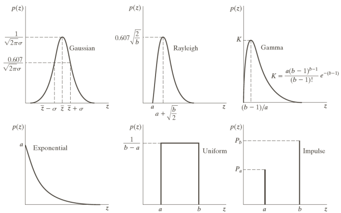
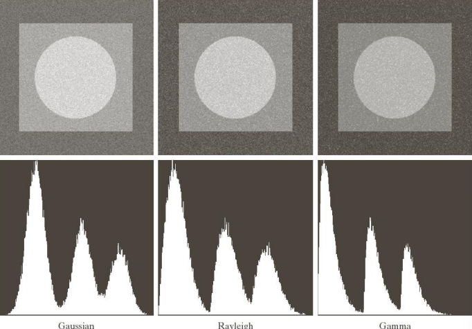
We can see the results of these noises by applying them on an image. Note that the impulse noise is the same as the salt and pepper noise.

We get
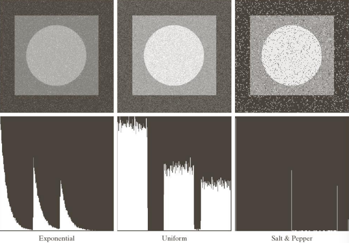
To restore such corrupted images we can use smoothing filters (eg. averaging and gaussian) or non linear filters (eg. median).
For example, let’s consider the original image (top left). We can corrupt is by using gaussian noise (top right), and then restore it by using arithmetic mean (bottom left) or geometric mean (bottom right)

Another possibility is to use the median filter (median: order the elements of a set, then choose the middle one). An interesting artefact of using the median filter is that we can reapply it multiple times over to get increasingly better results. For example, the corrupted image with salt and pepper (top left) is then reconstructed by applying the same median filter 3 times

Other averaging filters that can be used to remove different kinds of noise are the following ones
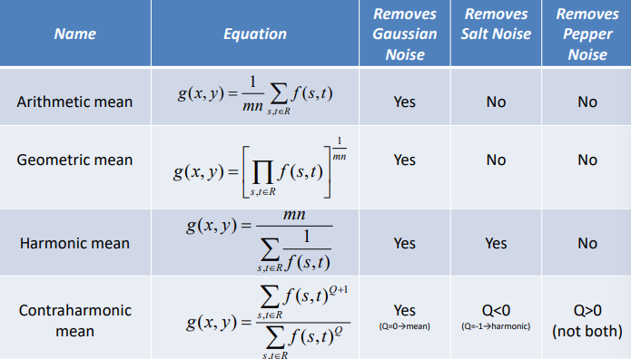
For example, by using the contrahrmonic filter to the image corrupted by pepper noise (top left) or salt noise (top right) [pepper noise only adds darker pixels, while salt noise adds white pixels and salt and pepper add both] we can remove salt noise with a negative value for Q (-1.5 in this case, bottom right), or a positive Q value to remove pepper noise (+1.5 in this case, bottom left).
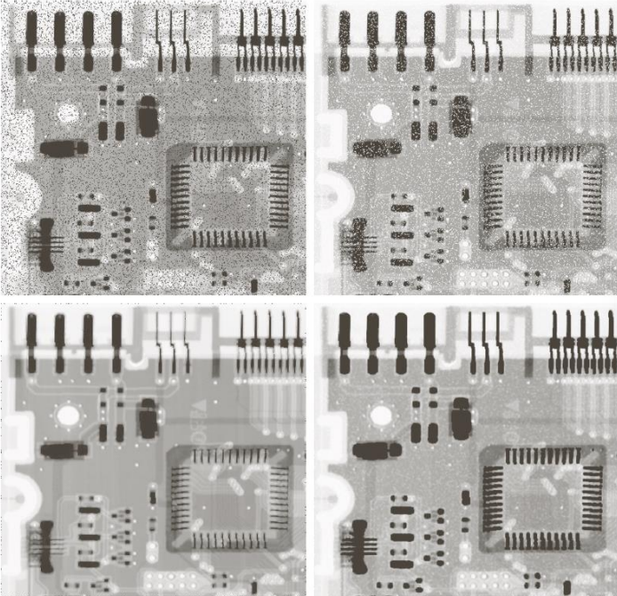
Max and Min filters
- Max filter: highlights salt noise while removing pepper noise (left)
- Min filter: highlights pepper noise, removes salt noise (right)
Referring to the top images of the previous image we get

Alpha-trimmed mean
The Alpha-trimmed mean is a statistical method used in image processing to reduce the influence of noise. It involves sorting the data, removing a certain percentage of extreme values (alpha percent from both ends of the sorted data), and then calculating the mean of the remaining values. This approach provides a robust estimation of central tendency by effectively filtering out outliers while preserving useful information in the dataset. The alpha parameter allows for adjusting the level of trimming, enabling flexibility in handling different degrees of noise or outliers. The Alpha-trimmed mean is commonly employed in image denoising, where it helps to improve image quality by suppressing unwanted artifacts without significantly distorting the underlying image structure.
For example, applying the concept of alpha trimmed mean to the following matrix, we can eliminate the extreme values and then calculating the mean of the remaining values
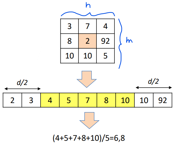
Mathematically, it coincides with
g(x, \, y) = \dfrac{1}{mn-d} \sum_{s, \, t \, \in \, R_r} f(s, \, t)From a practical standpoint, we can see that the alpha-trimmed median filter yields the best result in the following scenario
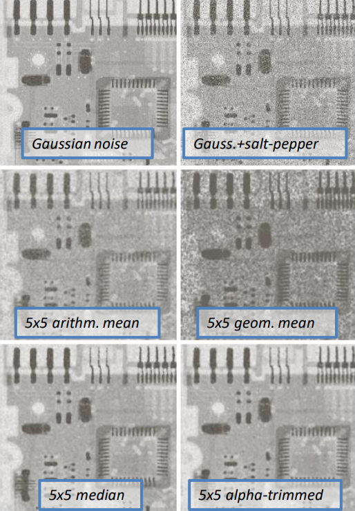
Note: the alpha-trimmed mean, in this case, uses d=5.
Adaptive filters
Adaptive filters are a class of filters widely used in image processing applications where the characteristics of the environment (the surrounding pixels) may change over time. Unlike traditional filters with fixed coefficients, adaptive filters dynamically adjust their parameters based on the input signal. This adaptability allows them to effectively track and respond to changes in the environment, making them particularly useful for tasks such as noise reduction. Adaptive filters utilize algorithms such as the least mean squares (LMS) algorithm or the recursive least squares (RLS) algorithm to continuously update their coefficients, optimizing their performance in real-time.
A general rule can be obtained by considering local image variance (\sigma_L^2) and the noise variance (\sigma_{\eta}^2). Local image variance represents the variability of pixel intensities within a local region of the image, while noise variance represents the level of noise present in the image. Specifically, when
- \sigma_{\eta}^2 \ll \sigma_L^2 the filter should be weak. In other words, in regions with strong image features such as edges or other important image elements, the filter’s effect should be minimal to avoid blurring or distortion of these features
- \sigma_{\eta}^2 \approx \sigma_L^2 the filter should be strong. In fact, in this case, the noise is comparable to (or even dominant) over the image content, therefore the filter should be strong and aggressive in reducing noise to enhance image quality and improve visual clarity
Visually, an adaptive filter can have a positive effect on overall image quality. By using a 7 \times 7 matrix we can see that geometric and arithmetic mean don’t perform as well (while keeping the matrix size constant, for different matrices the results might differ).
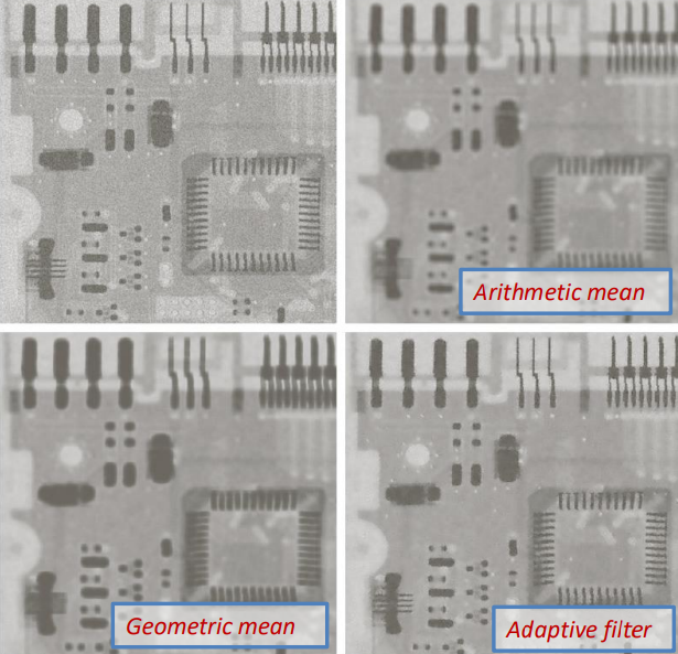
Similarly, in the case of salt and pepper noise the median filter performs better in reducing the noise. The downside of adaptive filters is their higher computational cost.


