Mid-level processing - Giacomo D`Andria

Table Of Contents

Edge detectors
Detecting edges using first order derivatives
Detecting edges with second order derivatives
Writing an edge detection algorithm
Notes:

After having seen the low level components of image processing, we can now move to mid level elements that utilize the tools seen so far, and by combining them create more advanced features for image processing.

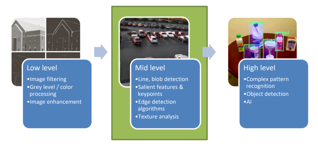
We’ll look into:

Edge detection
Line detection

Edge detectors

Edge detectors highlight edges in an image. Specifically, an edge can be caused by a variety of factors, for example

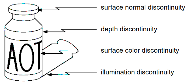
We will use derivatives, specifically gradients and Laplacians. We’ll use them to find different features of the edges

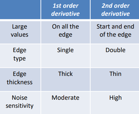
For example

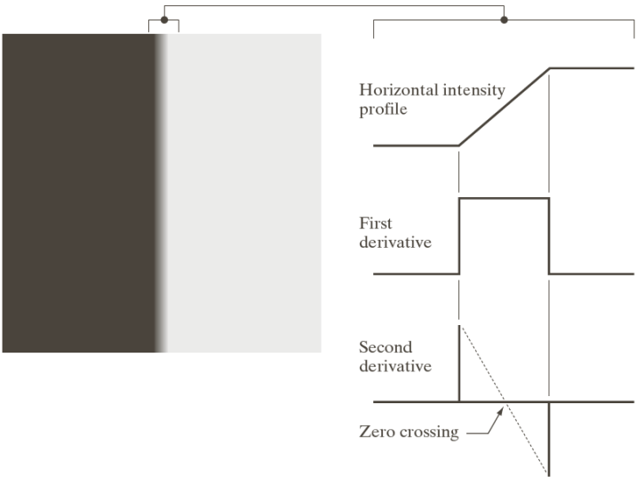
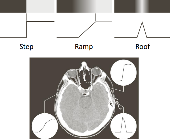
First and second order derivatives examples

We can furthermore divide the edges into different kinds with respect to the gradient shape

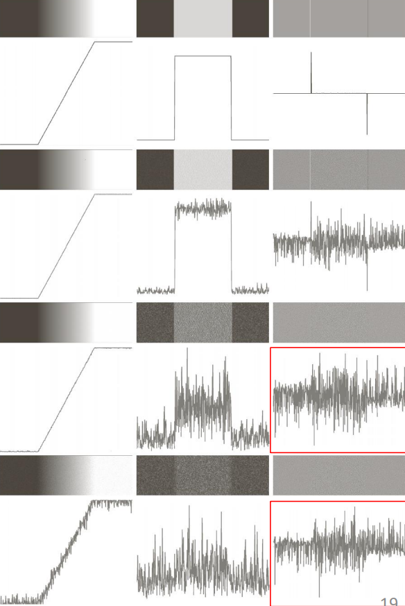
Note: derivatives amplify the noise—2nd derivatives more than 1st.

Detecting edges using first order derivatives

What is a gradient and first order derivatives: In the continuous case

\nabla f(x, \, y) = \left[\dfrac{\partial f}{\partial x}, \, \dfrac{\partial f}{\partial y}\right] := [g_x, \, g_y]

While in the discrete case

g_x = f(x+1, \, y) - f(x, \, y)\\ g_y = f(x, \, y+1) - f(x, \, y)

The gradient points towards the fastest varying direction.

By considering the magnitude and the phase of the gradient, we can infer information about edge features

\begin{aligned} &\text{Magnitude:}&&||\nabla f(x, \, y)|| = \sqrt{g_x^2+g_y^2}\\[10pt] &\text{Phase:} && \alpha := \theta = \tan^{-1}\left(\dfrac{g_y}{g_x}\right) \end{aligned}

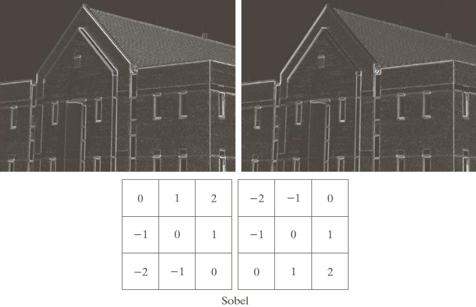
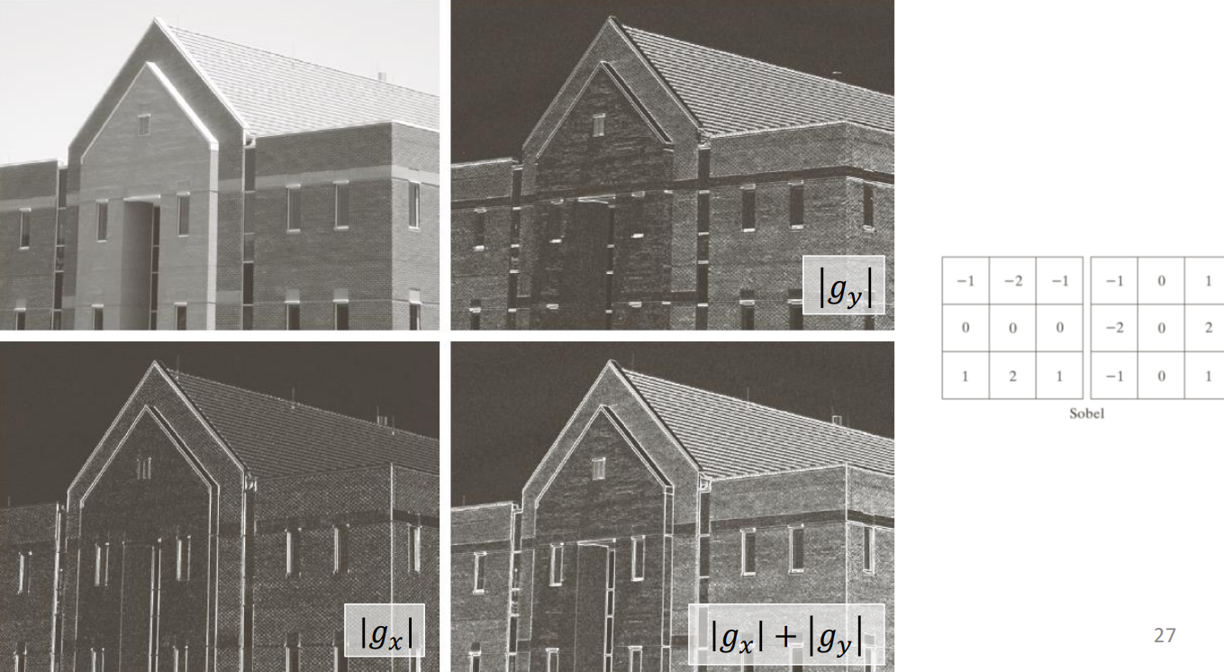
By using gradient masks and the Sobel operator, we can detect edges in multiple directions. The Sobel edge detector is named after its inventor, Irwin Sobel, this operator utilizes convolution with a pair of small, separable filters to compute the gradient magnitude of an image, effectively pinpointing regions of significant intensity variation. By detecting abrupt changes in pixel intensity, the Sobel edge detector offers valuable insights into the structure and boundaries of objects within an image.

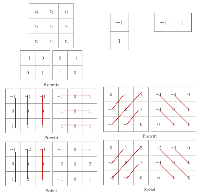
Through the usage of Sobel filters we can therefore detect edges along $x$ and $y$ directions, as well as in the diagonal directions. An example usage is shown below using the magnitude as the edge detection

If we were to use the angle we would get the following image

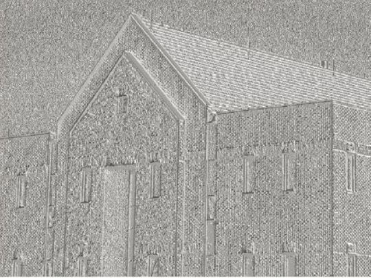
In which areas with the same intensity have similar features.

Detecting edges with second order derivatives

What is a Laplacian and second order derivatives: In the continuous case, the Laplacian is

\nabla^2 f(x, \, y) = \dfrac{\partial^2f}{\partial x^2} + \dfrac{\partial^2 f}{\partial y^2}

Where

\dfrac{\partial^2 f(x, \, y)}{\partial x^2} = f(x+1, \, y) + f(x-1, \, y) - 2f(x, \, y)

In the discrete domain

\nabla^2 f(x, \, y) = f(x+1, \, y) + f(x-1, \, y) + f(x, \, y+1) + f(x, \, y-1) -4f(x, \, y)

Visually, applying the Laplacian to detect edges, we get

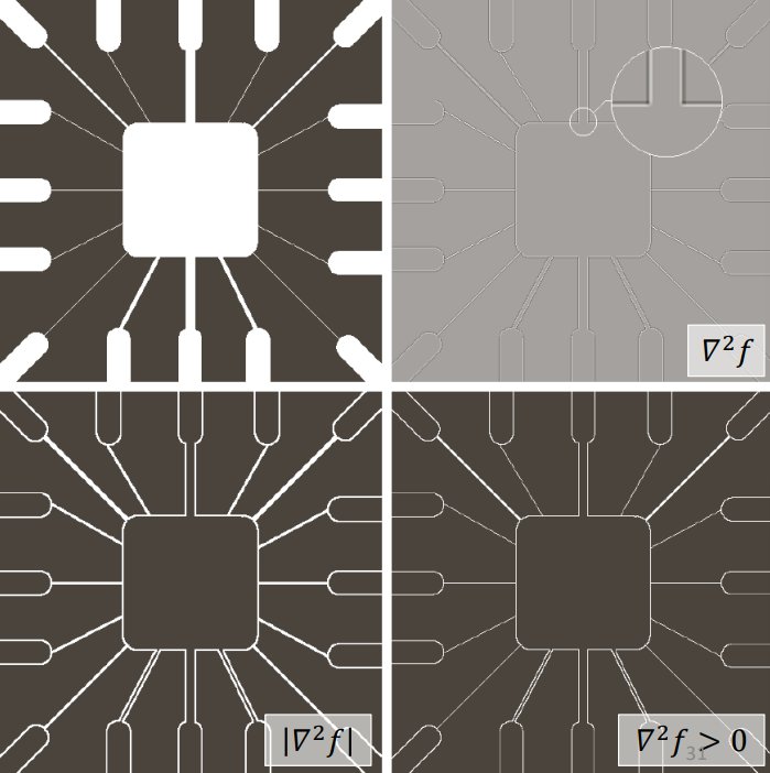
Laplacian filter can be used to detect edges

From the Laplacian, we can derive the anisotropic detectors, which offer four available directions

And can be used to detect edges in a certain direction. In the following example at 45 degrees.

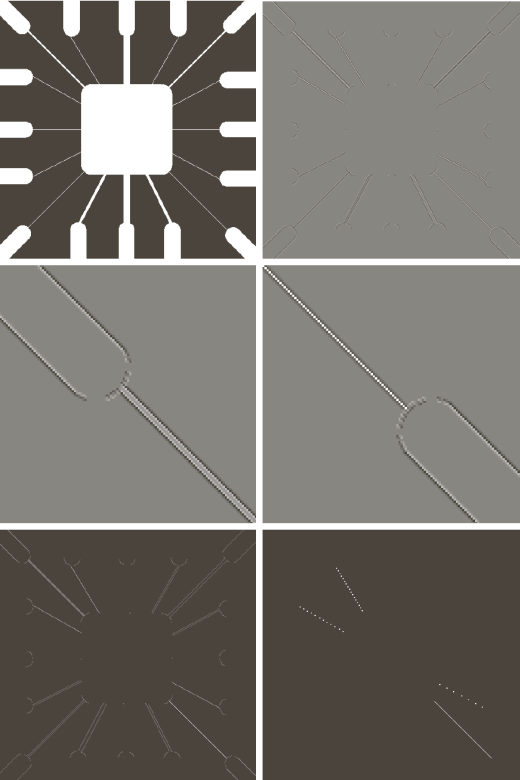
Note: images in the middle are zoomed in views of the top left and bottom right region, while image on the bottom left has all negative values set to 0 and image on the bottom right has some points set to white that are above a certain threshold given by the other image next to it.

Writing an edge detection algorithm

Apply low-pass filter for noise removal
Calculate gradient
Apply gradient thresholding, specifically $|\nabla f| > T$

The final result is shown in the bottom right image:

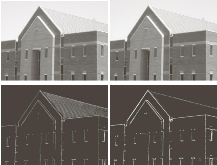
Notes:

The effect of smoothing is often useful prior to the computation of the gradient to minimize the amount of “wrong edges” that are detected

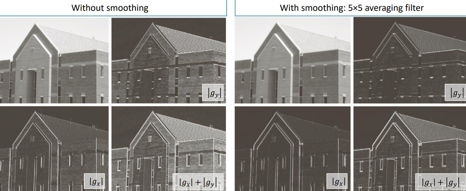
By applying thresholding we can separate the stronger edged from the others. The final effect depends on the amount of smoothing applied as well

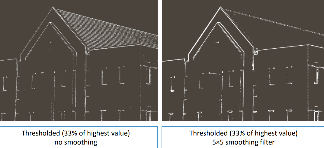
We can then calculate the diagonal edges by using Sobel filters

Detecting diagonal edges with sobel filter

Did you find this article interesting?

YesNo