Single pixel operations, also known as point operations or pixel-wise operations, are fundamental operations in image processing where individual pixels in an image are independently manipulated. These operations are essential for basic image enhancement, correction, and manipulation. Common single pixel operations include adjusting brightness, contrast, and gamma, as well as performing thresholding and color space conversions.
Let’s consider a simple example using a grayscale image. This image has L gray levels (commonly 256, but this number could vary), through the use of single pixel operations we can change the gray levels of the image. Specifically, we’ll need to represent the content of the picture using a function I(x, \, y) and another function T(\cdot) that represents the gray level change.
What we first need to do is read the value of the pixel, than we apply the transformation, and then we override the original pixel with the newly modified one.
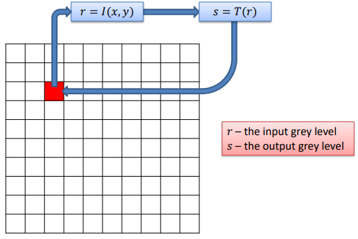
Some of the operations that can be done this way are:
- Negative
- Logarithm
- Gamma
- Contrast stretching
- Intensity slicing
- Histogram equalization
But are not limited to those ones.
Negative / Logarithm / Gamma transformations
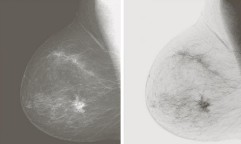
The negative transformation switches dark and light areas of an image. It is represented mathematically by
s=(L-1)-r
Where L represents the total number of gray levels of the image, while r is the specific gray value of the layer that is being currently considered.
The log transform highlights the differences among pixels in given conditions, which enhances the difference in the image, revealing some of the details. It is represented by
s = c \log(1+r),\underbrace{c=\dfrac{L-1}{\log(L)}}_{\displaystyle\text{Normalization constant}}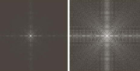
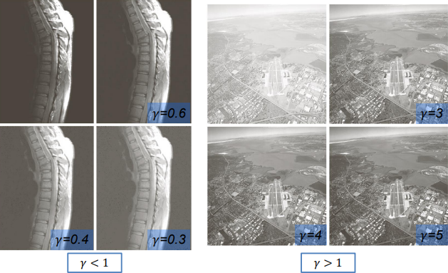
The gamma transform is very similar to the log transform, but the difference is that we can tune this function by adjusting the gamma (\gamma) parameter and make the image lighter or darker depending on its value. Mathematically, it is
s=cr^{\gamma}, \qquad c=(L-1)^{1-\gamma}Which has different curves based on gamma
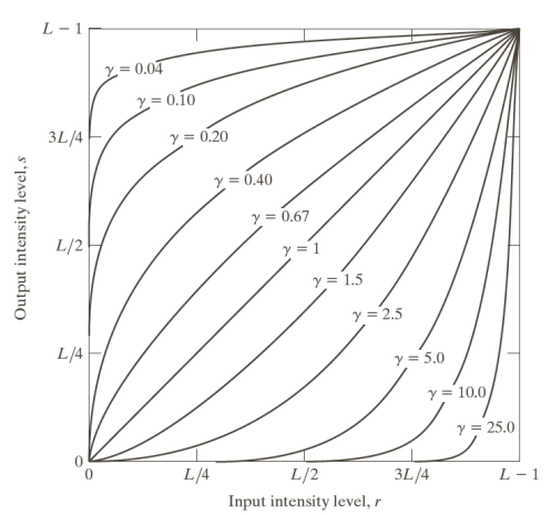
And produces different outputs
Contrast stretching
Through single pixel operations we can enhance the contrast in an image by trying to “stretch” the values into a specific contrast range. We might want to extend or compress such range depending on what our goals are. As seen in a previous lesson, contrast is the difference between the highest and lowest intensity levels in an image. To measure it, we can use the so called RMS (Root Mean Square) contrast
RMSC = \sqrt{\dfrac{1}{MN} \sum_{i=0}^{N-1} \sum_{j=0}^{M-1}\left(I(i, \, j) - \bar{I}\,\right)^2}In words: the formula calculates the Root Mean Square Contrast by summing up the squared differences between each pixel’s intensity and the average intensity across all pixels in the image. This sum is then normalized based on the image dimensions (rows and columns), and the square root is taken to obtain the final result. RMSC is a measure of the overall contrast or variability in pixel intensities within an image.
In which the terms mean:
- \dfrac{1}{MN}: This term represents the reciprocal of the product of the number of rows (M) and the number of columns (N) in the image. It is used to normalize the result based on the image dimensions.
- \displaystyle\sum_{i=0}^{N-1}: This signifies a summation operation over the rows of the image. The variable i ranges from 0 to N-1, where N is the number of rows.
- \displaystyle\sum_{j=0}^{M-1}: Similarly, this represents a summation operation over the columns of the image. The variable j ranges from 0 to M-1, where M is the number of columns.
- I(i, \, j): This is the intensity value of the pixel located at the i-th row and j-th column of the image.
- \bar{I}: This denotes the average intensity value of all pixels in the image.
- \left(I(i, \, j) - \bar{I}\,\right)^2: This is the squared difference between the intensity value of a specific pixel and the average intensity value of the entire image.
Thresholding
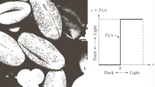
With thresholding we divide the pixels of the image into black and white, rounding each of them to the closes extreme value.
Applying Contrast stretching & Thresholding
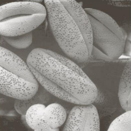
Suppose we want to increase the contrast of this image

We can apply the following filter to compress the darker and lighter values and stretch (give more space) to the middle tones
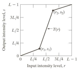
The output we get is a much clearer image
By applying the thresholding, we simplify the image flattening it by applying the filter on the right and getting two tones only
Bit plane slicing & intensity slicing
These effects, although not very popular, can be useful in certain cases when only a subset a specific range of gray levels should be considered in a given image. We can distinguish between:
- Intensity slicing: considers only a subset of the gray levels setting all the others to white or black.
For example, by using the following transformations
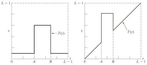
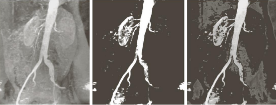
We can highlight the intensities in the range [A, \, B] and reduce all others (left image) or highlight the range [A, \, B] and keep all others with varying levels of intensity (right image).
For example, by using the first transformation we get the image on the left, while using the second one we get the one on the right
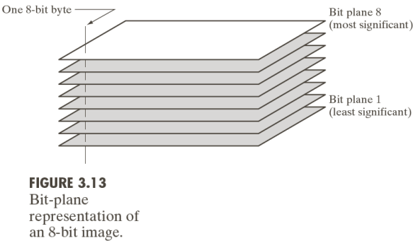
- Bit plane slicing: considers only a subset of the bits that encode the gray levels. Considering a bit-plane representation of an 8-bit image we can in fact represent it as
By adding more and more bits to the representation of the top left image below, we add one bit at the time until we get the representation of in the bottom right. Therefore, we start off with what looks like white noise, then, by adding an increasing number bits to represent the information encoded in the gray levels, we end up with the bottom right image that uses 7 out of 8 total bits.
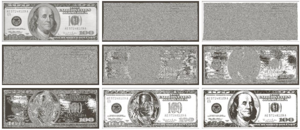
Using bit planes we can also reconstruct images. For example, going from left to right we add more layers to the reconstruction to get a better looking image

Histogram equalization
Histogram equalization is technique in computer vision used for enhancing the contrast and improving the visual quality of digital images. The concept revolves around the distribution of pixel intensities within an image, represented by its histogram. In essence, histogram equalization aims to transform the intensity values of pixels in such a way that the resulting image has a more uniform or equalized histogram.
The process involves redistributing the pixel intensities across the entire dynamic range, stretching the original distribution to cover a wider spectrum. This is achieved by mapping the input intensities to new values using a specific transformation function. As a result, regions of the image with initially lower contrast become more distinguishable, leading to a visually improved representation.
For example, if the distribution is similar to the one below
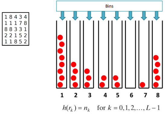
We know there is gonna be a prevalence of the pixels at the two extremes. Normalizing the image turns those imbalances into a better distributed set, in which all bins have a similar amount of pixels in them.
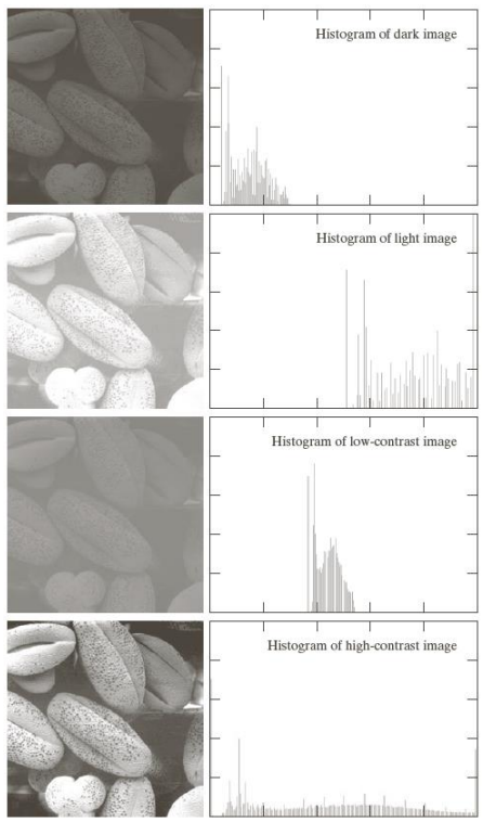
We can take a look at the following images and their histograms to see the different distributions in pixel density
To mathematically calculate the probability p(\cdot) of a particular pixel having intensity r_k, we can consider
p(r_k) = \dfrac{\textcolor{05D9E8}{h(r_k)}}{MN}=\dfrac{n_k}{MN}In words: The formula calculates the probability of a particular pixel intensity r_k occurring in the image. It does so by dividing the count of pixels with intensity r_k (equivalently, n_k) by the total number of pixels MN in the image (M is the number of rows and N is the number of columns). This probability distribution is often used in image processing and computer vision, providing insights into the relative frequencies of different pixel intensities within an image.
Modifying the histogram
We can modify the histogram to equalize it based on an equalization function to flatten it. By considering p(r_k) as a Probability Density Function (PDF) we can equalize it by using T(r), a monotonically non-decreasing function, therefore continuous and differentiable. The function T(r) is constrained to the range [0, \, L-1], where L is the number of possible intensity levels in the image. Additionally, r is constrained to the same range [0, \, L-1]. These constraints maintain the integrity of the pixel intensities throughout the histogram equalization process. They prevent the transformation function from producing invalid or out-of-range intensities.
CDF and PDF recap
The Cumulative Distribution Function (CDF) is defined as
F_X(x) = P(X \leq x)
While the Probability Density Function (PDF) is
f_X(x) = \dfrac{d}{dx} [F_X(x)]From which we can get
F_X(x) = \int_{-\infty}^x f_X(t) \, dtThe CDF is the T(r) transformation used to equalize the histogram
s = T(r) = (L-1) \int_0^r p_r(w) \, dw\\[10pt]

s_k = T(r_k)=(L-1) \sum_{j=0}^k p_r(r_j)
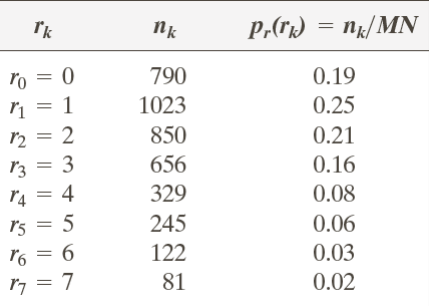
For example, we can consider a 3-bit case that has |r_k|=2^3=8 levels that, using the aforesaid formulas, lead to the construction of the following table:
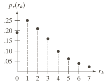
To which corresponds the following histogram with a clear left-values majority
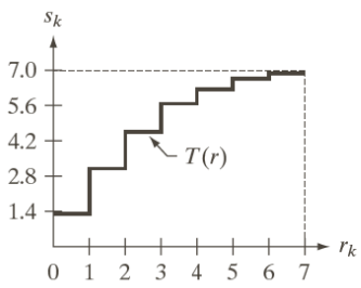
To create the transformation function we can use the formula
s_i = 7 \sum_{j=0}^i p_r(r_j)With which we can build the following table of values
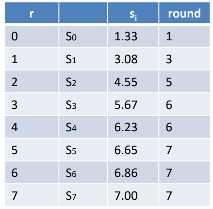
That correspond to the transformation function T(r) below
By equalizing the original histogram with the transformation function we get
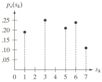
Which is the flattened histogram.
Note: because of the few levels that are being used to flatten it the result is not exactly a flat histogram, but by using more levels the approximation would get better and better.
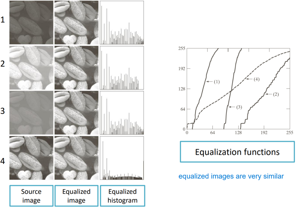
Other examples are reported below, where on the right there are the relative equalization functions.
Histograms in OpenCV
void cv::calcHist(
CV::InputArrayOfArrays images, // vector of 8U or 32F images
const vector<int>& channels,   // lists channels to use
CV::InputArray mask,           // in 'images' count, iff 'mask'
                               // nonzero
CV::OutputArray hist,          // output histogram array
const vector<int> histSize,    // hist sizes in each dimension
const vector<float>& ranges,   // pairs give bin sizes in a
                               // flat list
bool accumulate = false        // if true, add to 'hist', else
                               // replace
);
Read the docs here.
Extensions of histogram equalization
The concept of histogram equalization can be extended to local histogram equalization, meaning we can apply different equalizations to different portions of the image and use multiple equalization functions.
For example, if different regions of the image have very different pixel distribution characteristics like below, the image on the left

If we just use a single histogram we get the image in the middle, but by using multiple functions we can extract more information and realize that there are symbols hidden in the various squares.
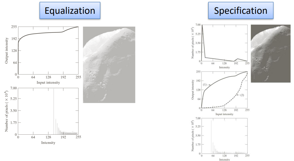
Another extension that we can use is the histogram specification, which allows us to choose the output structure of the final histogram, without only flattening it. To get this result, we firstly need to specify the desired output shape of the histogram, from which we can obtain the inverse transformation and then apply it to an equalized histogram to change its structure.
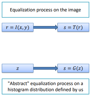
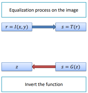
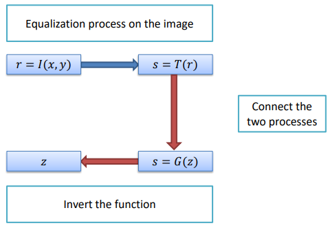
The mathematical formulation of this procedure is as follows:
- We need to calculate the transformed intensity values s_k from the input image
s_k = T(r_k) = (L-1) \sum_{j=0}^k p_r (r_j)In words: for each pixel intensity r_k in the input image, we use the function T(\cdot) to get the transformed intensity and scale it in the accepted range (L-1). Specifically, the summation represents the probability of encountering a pixel with intensity r_j in the input image. In simpler terms, the formula calculates the transformed intensity s_k by considering the cumulative probability of encountering pixel intensities up to r_k. The cumulative sum is weighted by the scaling factor (L-1) to ensure the result is within a valid intensity range.
- Then, we can define the desired output Probability Mass Function (PMF) p_z(z_i) and evaluate the corresponding Cumulative Distribution Function (CDF) G(\cdot) for target s
s=G(z_q) = (L-1) \sum_{i=0}^q p_z(z_i)- At this point, we can obtain the inverse transformation, namely the mapping from s to z
z_q = G^{-1} (s_k)- Finally we can equalize the input image (r\to s) and apply the inverse mapping z=G^{-1}(s). We are therefore equalizing the input image by replacing each pixel intensity r with its corresponding transformed intensity s and then afterwards applying the inverse mapping to obtain the equalized image in accordance with the desired output distribution.
For example, if we want to get the histogram on the right from an image that has the histogram on the left
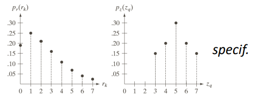
We would need to use the various equations to calculate the equalized values of the input image (left table), and then calculate the new value for the pixels based on the specified histogram (right table).

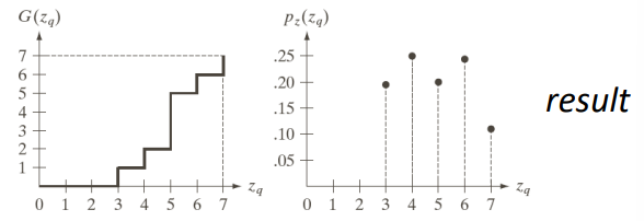
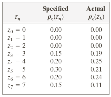
At this point, the representation of the inverted function G(\cdot) is on the left, while the new obtained histogram distribution is on the right, while the actual values of the specified and obtained values is below.
In a real-life scenario, from an image with an unbalanced histogram
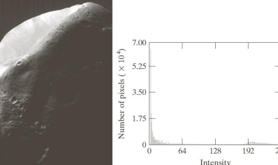
We can first equalize it, and then change the histogram based on our desired effect
