The Canny edge detector represents a cornerstone in the field of computer vision and image processing, renowned for its robustness and effectiveness in detecting edges within digital images was developed by John Canny in 1986. This edge detection algorithm aims to accurately locate edges while minimizing the impact of noise and spurious responses. By employing a multi-stage process involving gradient computation, non-maximum suppression, and edge tracking by hysteresis, the Canny edge detector excels in identifying edges with high precision and low false positive rates. Its adaptability to varying image conditions and ability to capture fine details make it a preferred choice for a wide range of applications, including object recognition, scene analysis, and image segmentation.
The canny algorithm works the following steps:
- Smoothing with a Gaussian filter
- Gradient computation (magnitude and phase)
- Quantize the gradient angles
- Non-maxima suppression
- Hysteresis thresholding
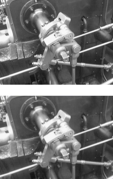
Step 1: smoothing
Firstly, the smoothing can be employed to reduce noise and better evaluate edges
Step 2: gradient computation
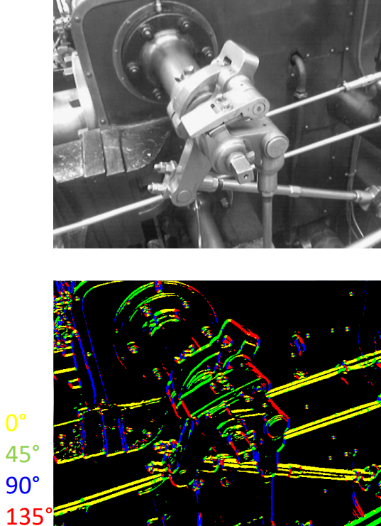
Edges are calculated using vertical, horizontal and diagonal masks by using the gradient equations already seen in the previous chapter
Step 3: edge quantization
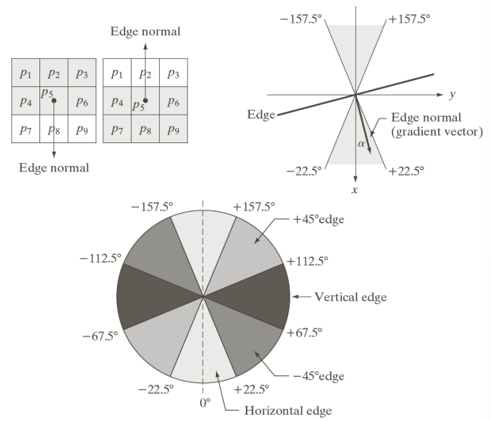
All identified edges have to be grouped into values that belong to the same range, usually that range is determined by 45 degrees increments.
Step 4: non-maxima suppression
Non maxima suppression reduces the edged thickness. Thin edges are in fact desirable to accurately locate an edge.
To obtain this, we have to first cross an edge, then we can select the strongest point in that edge. From a practical standpoint, if the current pixel’s value is not larger than at least one of its neighbors in the gradient direction, then the pixel’s value is set to zero. This has the effect of thinning the edges down to single-pixel width.
The number of pixel neighbors differs according to the intended usage. If we consider a 3 \times 3 matrix, the center pixel has 8 neighbouring other pixels
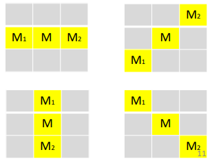
Usually, the number of quantized directions is either 8 or 16.
Step 5: hysteresis thresholding
Hysteresis thresholding is used to keep strong edges and week edges connected with strong ones while rejecting isolated weak edges. The edge strength is measured by means of gradient magnitude.
Two thresholds are chosen: a high threshold T_H and a low threshold T_L.
- Pixels with gradient values above T_H are classified as strong edge pixels.
- Pixels with gradient values between T_L and T_H are considered as weak edge pixels.
- Pixels with gradient values below T_L are discarded as non-edge pixels.
Once we’ve identified strong and weak edge pixels based on the dual thresholds, we proceed to ensure that weak edge pixels that are adjacent to strong edges are also classified as part of the edge.
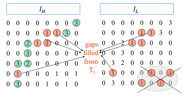
Visual representations of the various steps
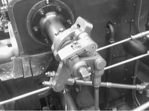
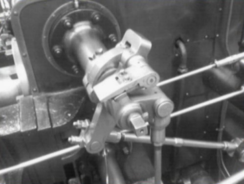
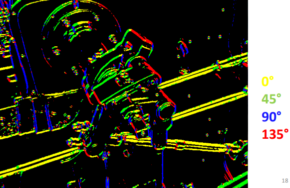
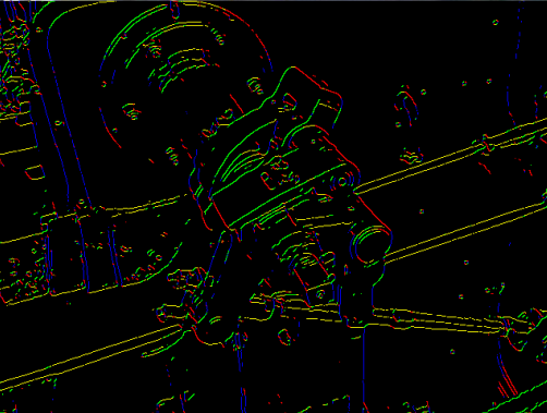

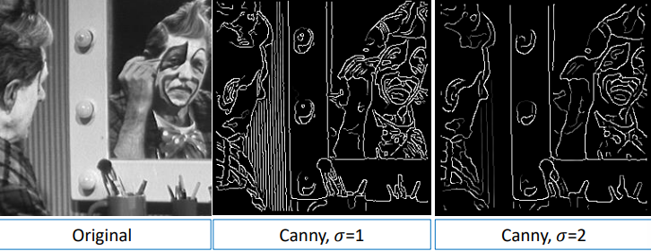
Observations on different effects
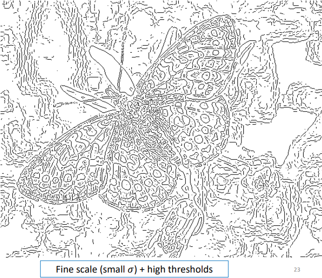
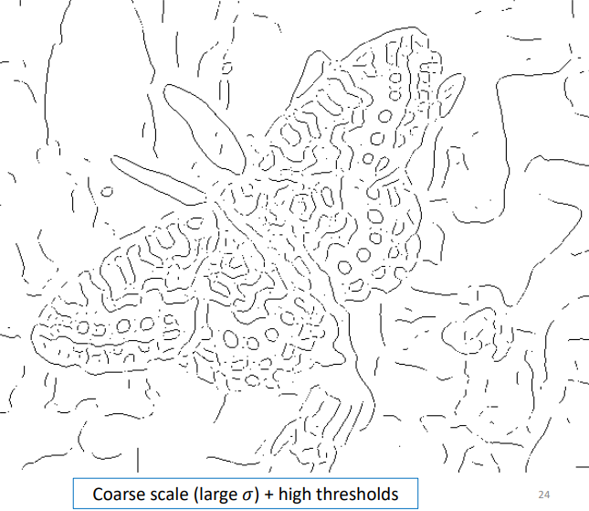
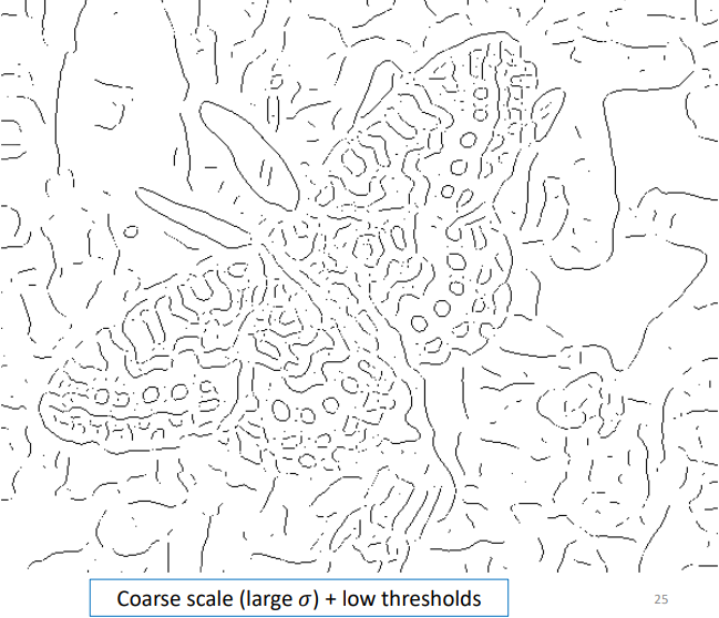
By using different kernels sizes (\sigma) for the gaussian smoothing we get different results of the detected edges. With smaller \sigma values we retain finer details.
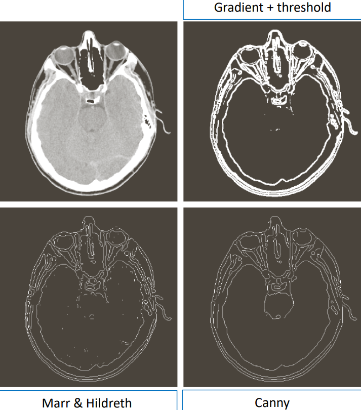
Another example

Other edge detectors
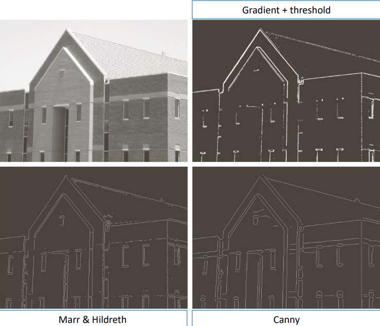
Different edge detectors yield different results in the amount of details and type of lines.
