The frequency domain refers to a mathematical representation of an image where the spatial information is transformed into frequency information. This transformation is typically achieved through techniques such as the Fourier Transform. In the frequency domain, images are decomposed into different frequency components, revealing patterns, textures, and structures that might not be readily apparent in the spatial domain. This domain shift is particularly valuable for tasks such as image analysis, enhancement, and filtering, as it allows for efficient manipulation and processing of image data based on their frequency characteristics. By analyzing images in the frequency domain, computer vision systems can extract meaningful features, suppress noise, and enhance image quality, thereby enabling more effective interpretation and understanding of visual information.
Firstly, we have to define a transform space in which to apply the Fourier transform by using the Fast Fourier Transform (FFT) algorithm. Because images have two dimensions, x and y, we need to transform them into two different frequencies:
x \to f_x\\
y \to f_y
Mathematically, the Fourier transform in 1D is
F(\mu) = \int_{-\infty}^{+\infty} f(t) \exp(-j2\pi\mu t) \, dtSimilarly, the inverse transform is
f(t) = \int_{-\infty}^{+\infty} F(\mu) \exp(j2\pi\mu t) \, d\muAn example of a transformed signal into the Fourier representation is the \texttt{rect} function, which, when transformed, becomes the \texttt{sinc} function. In addition to the transformed signal, the spectrum is also and interesting function that can be obtained by getting the absolute value of the transformed signal.

Because we cannot digitally represent continuous functions, we can use a set of regular pulses separated by \Delta t time between them to sample the original signal. Practically speaking, such sampling happens by multiplying the impulses with the function
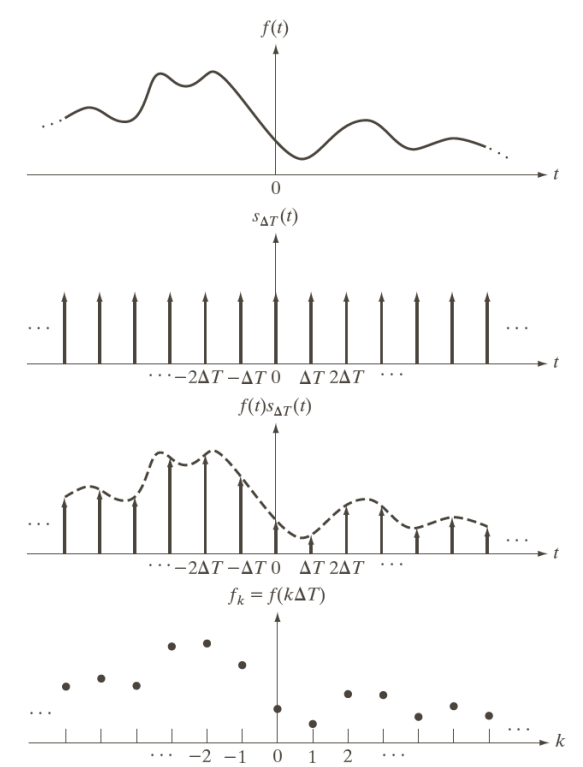
The impulses are expressed by means of the Dirac delta function, defined mathematically as
\delta(t) =
\begin{cases}
\infty & \text{if } t=0\\
0 & \text{if } t \neq 0
\end{cases}
Features of the Dirac delta function are:
- Unit area
\int_{-\infty}^{+\infty} \delta(t)\,dt=1- Sifting property in 0
\int_{-\infty}^{+\infty} f(t)\cdot\delta(t)\,dt=f(0)- Sifting in a generic position
\int_{-\infty}^{+\infty} f(t)\cdot\delta(t-t_0)\,dt=f(t_0)The second two points “select” a specific point in the function!
When discrete variables are involved, the Dirac function can be expressed simply as
\delta(t) =
\begin{cases}
\infty & \text{if } t=0\\
0 & \text{if } t \neq 0
\end{cases}
Which automatically satisfies
\sum_{x=-\infty}^{+\infty} \delta(x)=1An impulse train is therefore expressed by a sum of delta functions
S_{\Delta t}(t) = \sum_{x=-\infty}^{+\infty} \delta(t-n\Delta T)And because the samples signal is the multiplication between the original signal and the train of impulses, we get
\tilde{f}(t) = \sum_{x=-\infty}^{+\infty} f(t) \cdot \delta(t-n\Delta T)In the transformed domain, the multiplication of the function with the impulses becomes a convolution
\widetilde{F}(\mu) = \int_{-\infty}^{+\infty} F(\tau) S(\mu - \tau) \, d\tauWhich we can transform (the calculations don’t matter) into
\widetilde{F}(\mu) = \dfrac{1}{\Delta T} \sum_{n=-\infty}^{+\infty} F\left(\mu-\dfrac{n}{\Delta T}\right)Note: this means that in the transformed domain, the spectrum is replicated, which in turn can generate an effect called aliasing.
Specifically, by sampling a band-limited function, can generate aliasing as
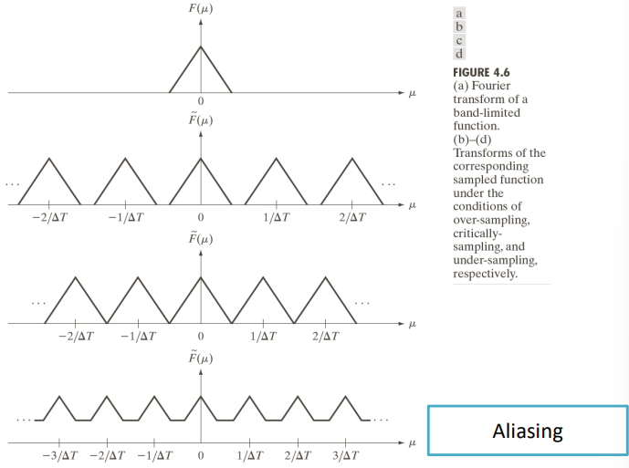
The sampling theorem states that the conditions under which we can reconstruct a signal is that the signal must be band limited, and
\dfrac{1}{\Delta T} > 2 \mu_{\text{max}}Where 2\mu_{\text{max}} is known as the Nyquist rate.
To reconstruct the signal we must isolate one repetition of the sampled signal by using a rect function
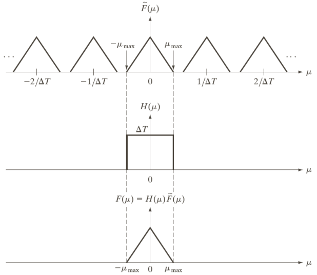
Images in the frequency domain
Images have some with respect to commonly used signals, namely images have 2 dimensions and only accept positive values for x and y. We therefore need Fourier transforms for the 2D space

Which extend into 3D space when they are represented into a graphical representation

Sampling can now be performed in both the x and y directions, which can lead to aliasing just like before
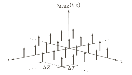
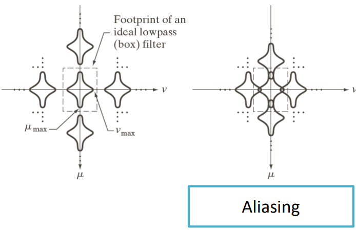
Similarly to what we did with the Nyquist rate, in 2D space the theorem becomes
F_X = \dfrac{1}{\Delta x} > 2 u_{\max} \quad\text{and}\quad F_Y = \dfrac{1}{\Delta Y} > 2 v_{\max}Where u_{\max} and v_{\max} at the maximum spatial frequencies of the signal along X and Y.
In this case, when we undersample an image (aka. we increase the \Delta x and \Delta y), we start to mess up the more detailed parts of the image—the lines in the example below.

To compensate for such effect, we can use a blurring filter. For example, by applying a 3\times 3 smoothing filter to the left image before undersampling the image, we can limit the effect of aliasing (right image).

In practical terms, aliasing takes place when the pixels’ color changes don’t align with round pixel values. In the images below, the length of the pixel changes, and (despite not being very visible) the aliasing effect is present.

Moiré effect
The Moiré effect pertains to a visual phenomenon that occurs when two patterns with a similar spatial frequency or grid structure are overlaid or superimposed. This overlapping creates interference patterns, resulting in the appearance of new patterns or distortions that were not present in the original images. In computer vision, the Moiré effect can pose challenges, particularly in tasks involving image analysis, pattern recognition, or optical character recognition (OCR).
Note: no aliasing is involved when dealing with this kind of effect.

Decomposing the discrete Fourier transform
The Discrete Fourier Transform (DFT) of an image can be decomposed into spectrum and phase.
F(u, \, v) = \underbrace{|F(u, \, v)|}_{\text{spectrum}} \cdot\underbrace{\exp(j \varphi(u, \, v))}_{\text{phase}}By distinguishing the real and imaginary parts of the transform we can rewrite them as
\begin{aligned}
&|F(u, \, v)| = \sqrt{R^2(u, \, v) + I^2(u, \, v)}\\[5pt]

&\varphi(u, \, v) = \tan^{-1}\left(\dfrac{I(u,\, v)}{R(u, \, v)}\right)
\end{aligned}
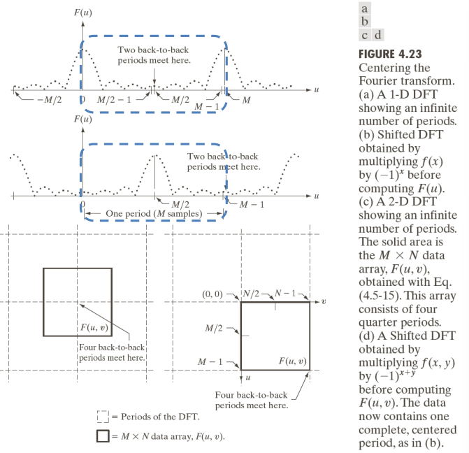
Usually, to center the Fourier spectrum, we have to move the Fourier spectrum (which stretches out both to the right and left with positive and negative values) to match up with the space where the image is represented.
Visually, visualizing the spectrum of the top left image we get the corners as being a little white. Centering the spectrum we can visually see that in the bottom left image the white spots are moved towards the center. Representing in using a log scale, the white spots are more prevalent over the vertical direction, as the original white rectangle was in that direction.
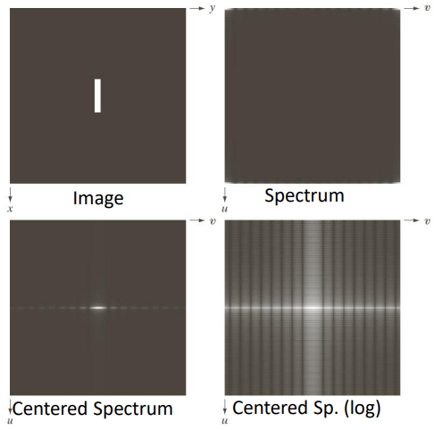
Note: the convention for the unit vectors u and v.
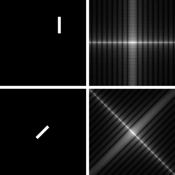
We can observe that by centering the spectrum, it doesn’t matter where the white piece is in the image, as it will always be centered in the spectrum view, at most it will be rotated like below
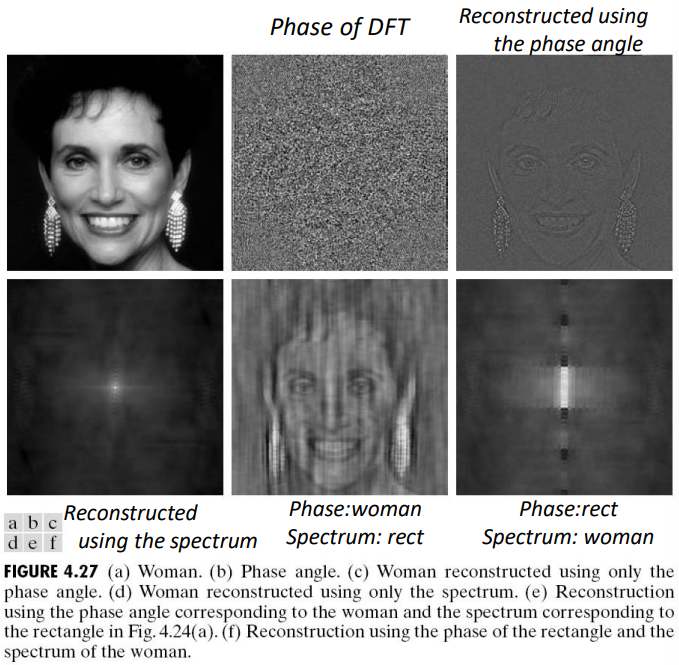
Information in spectrum vs phase
Both the spectrum and the phase encode information. The content encoded using the phase is able to retain more information than the information retained by using the spectrum.
Low-pass and high-pass filters
Low-pass filters
Filters can also be described in the frequency domain. Sometimes, it is easier to separate noise from the rest of the image in this domain. The necessary steps required to create filters in the frequency domain are

We will analyse the following
- Low-pass filters (smoothing):
- Ideal
- Butterworth
- Gaussian
- High-pass filters (sharpening):
- Ideal
- Butterworth
- Gaussian
Additionally, we will also take a look at selective filters, specifically:
- Band-reject
- Notch
Ideal low-pass filter
The Ideal low-pass filter serves as a fundamental tool for enhancing and manipulating digital images. This filter is designed to selectively pass or attenuate frequency components within an image. By allowing only low-frequency information to pass through while suppressing high-frequency noise, the Ideal low-pass filter facilitates tasks such as image smoothing, edge detection, and feature extraction.
This filter considers the concept of distance D from the center, letting through only some of the frequencies, and setting all the others to zero.

Using parametrized coordinates we can express that filter as a 2D function rotating on its axis
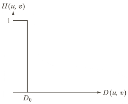
\begin{aligned}
&H(u, \, v) =
\begin{cases}
1&\text{if } D(u, \, v) \leq D_0\\
0&\text{if } D(u, \, v) > 0
\end{cases}\\[15pt]

&D(u, \, v) = \sqrt{\left(u-\frac{P}{2}\right)^2+\left(v-\frac{Q}{2}\right)^2}
\end{aligned}
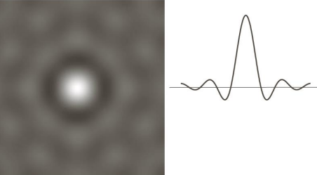
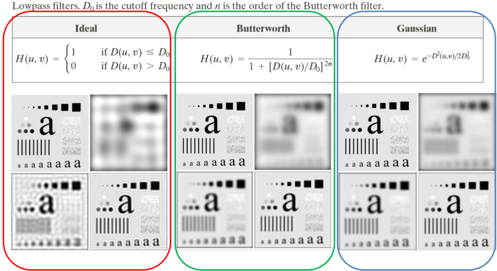
When considering the filter in space, the Ideal Low Pass Filter (ILPF) is implemented using matrices, but instead of having a sharp cutoff between the frequencies, in the spatial domain the filter generates ripples
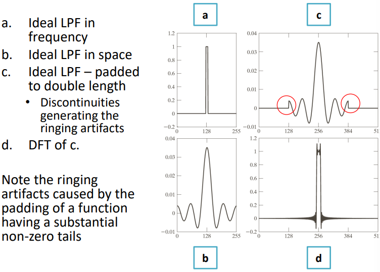
When applying the DFT those ripples generate artefacts
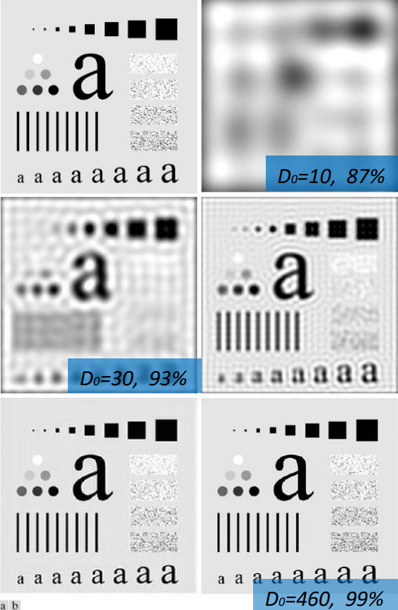
Visually, we can consider the original image (left) and its Fourier spectrum (right, resized to half the real size to match the original image). The circles correspond to 87%, 93.1%, 95.7%, 97.8% and 99.2% of the padded image power.
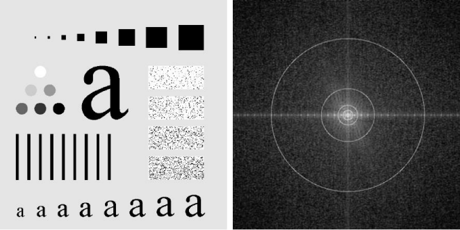
Removing the aforesaid percentages (specifically, the removed portion is 100 minus the said percentage), we get the following images:
Butterworth low-pass filter
The Butterworth low-pass filter stands as a tool for enhancing and analyzing digital images. Named after the British engineer Stephen Butterworth, this filter belongs to the family of infinite impulse response (IIR) filters and is renowned for its smooth and gradual attenuation of high-frequency components while retaining the essential low-frequency information within an image. Offering adjustable parameters such as cutoff frequency and filter order, the Butterworth filter provides flexibility in tailoring its response to suit various image processing tasks, including noise reduction, image smoothing, and feature extraction.
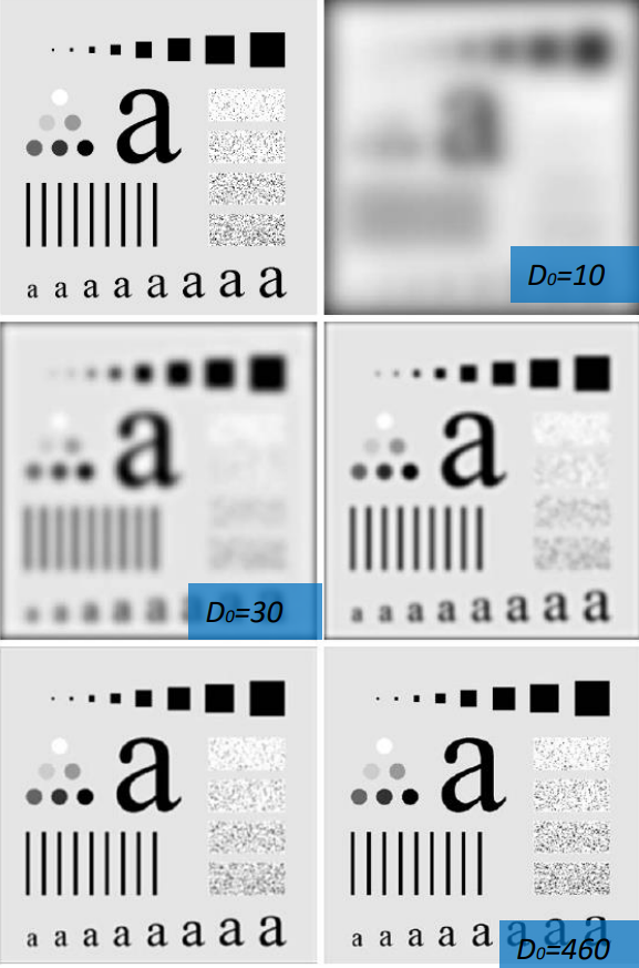
We can call the parameter to be tuned n. Large values of n cause this filter to be similar to the ILPF. Mathematically, we can represent it as

H(u, \, v) = \dfrac{1}{1+\left(\dfrac{D(u, \, v)}{D_0}\right)^{2n}}In the spatial domain, depending on the value of n we get different amounts of ringing effects.
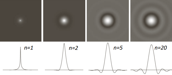
Visually, using n=1, \, \dots, \, 5, we get the following images
Gaussian low-pass filter
The Gaussian low-pass filter is derived from the Gaussian distribution, this filter is renowned for its ability to smoothly attenuate high-frequency components while preserving essential low-frequency information within an image. By convolving the image with a Gaussian kernel, the filter effectively reduces noise and blurs image details, facilitating tasks such as image smoothing, edge detection, and feature extraction. Its key advantage lies in its simplicity and computational efficiency, making it a popular choice for a wide range of image processing applications. With parameters like standard deviation controlling the extent of smoothing, the Gaussian low-pass filter offers flexibility to adapt its response according to specific image processing requirements.
Mathematically, it can be expressed as

H(u, \, v) = \exp\left(\dfrac{-D^2(u, \, v)}{2D_0^2}\right)Note: there is no ringing nor rippling effect in the filter.
Varying the values of \sigma = D_0 we visually get
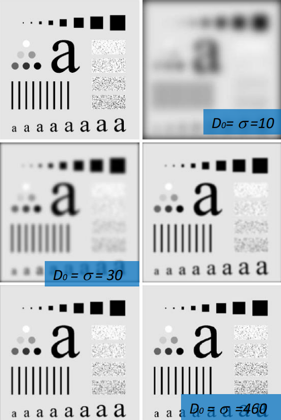
Applying the filter can fill gaps in the image thanks to its smooth shape

And for this reason it can be used as a “beautifying” filter to smooth skin features
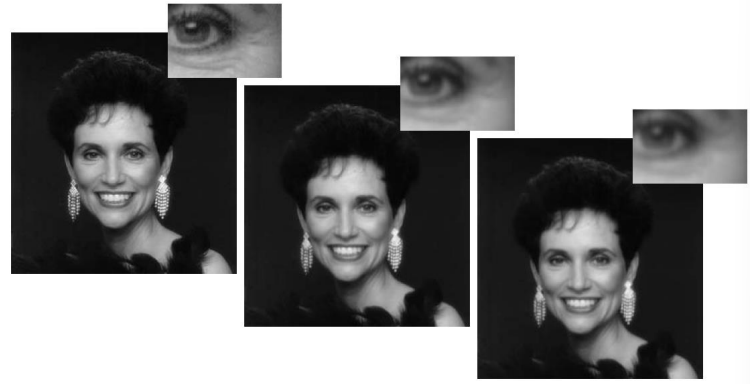
Similarly, it can be used to reduce noise by smoothing the image

Summary of low-pass filters
High-pass (HP) filters
The different version of the high-pass filters can be obtained by subtraction from the low-pass ones. Specifically
H_{\text{HP}}(u, \, v) = 1- H_{\text{LP}}(u, \, v)All those filters have similar features and create similar artefacts to the low-pass counterparts.
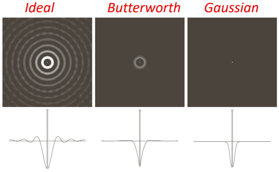
In the frequency domain the filters have the following shapes

While in the spatial domain
Visually, the ideal high-pass is shown below, with values D_0 = 30, \, 60, \, 120

While the Butterworth high-pass with the same D_0 values is

And the gaussian high-pass

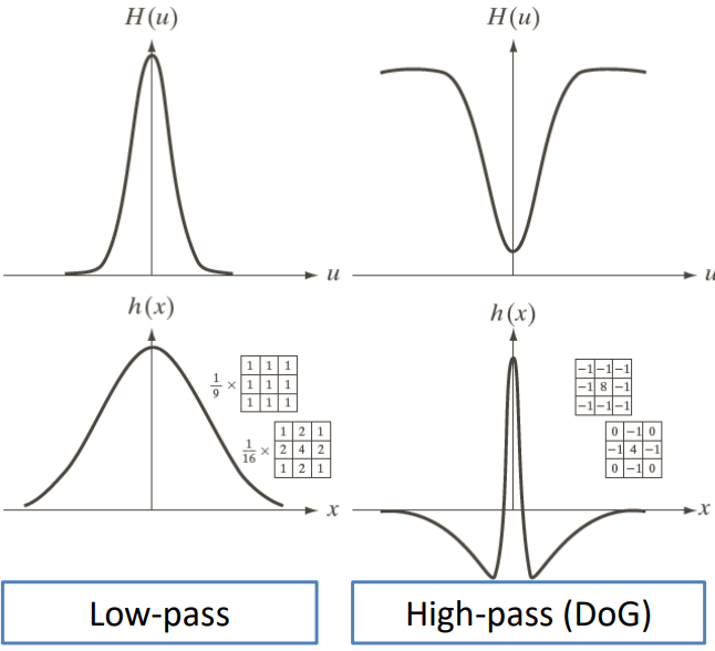
The spatial mask, a matrix or kernel utilized in spatial domain, is obtained by applying the inverse Fourier transform.
Selective filters
Selective filters work by selectively modifying specific features or components within the image. Unlike conventional filters that uniformly affect all parts of an image, selective filters are designed to target and manipulate particular regions or attributes, such as edges, textures, or colors, based on predefined criteria. These filters offer a nuanced approach to image enhancement, enabling practitioners to isolate and modify specific elements while preserving others, thus providing greater control over the visual outcome.
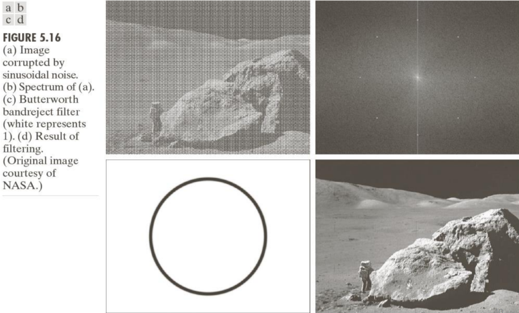
For example, in the presence of noise, there could be some frequencies that are particularly affected, therefore, selectively removing such frequencies could improve the overall quality of the image.

There are two categories of this kind of filters: band-pass and band-reject, and both of them use the same mathematical profiles we have seen for the previous filters.
Regarding the band-reject ones
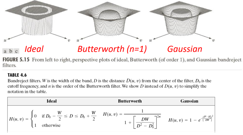
Which translate to the band-pass filters by subtraction:
H_{\text{bp}}(u, \, v) = 1 - H_{\text{br}}(u, \, v)Example usage of band reject filters if the following
Notch filters
Notch filters offer specialized capabilities for isolating and suppressing specific frequency components within digital images. Unlike traditional low-pass or high-pass filters that target broad frequency ranges, notch filters are engineered to selectively attenuate or eliminate narrow frequency bands, often associated with unwanted artifacts such as periodic noise or interference patterns. For example, in the top image there is an ideal notch filter, bottom left Butterworth of order two, on the right gaussian notch reject

The notch filters can lead to very complicated filters to remove noise on multiple frequencies. For example, by using
H_{\text{NR}}(u, \, v) = \prod_{k=1}^4 \left[\dfrac{1}{1+\left(\dfrac{D_{0k}}{D_k(u, \, v)}\right)^{2n}}\right]\cdot\left[\dfrac{1}{1+\left(\dfrac{D_{0k}}{D_{-k}(u, \, v)}\right)^{2n}}\right]We get the filter on the bottom left, which removes the noise of from the spectrum on the top right

Notch filter, in the space domain, have similar characteristics to the ones previously seen (as they are unions of multiple other filters).
The bilateral filter
The bilateral filter is a non-linear, edge-preserving, and noise-reducing smoothing filter for images. It combines gray levels on both their geometric closeness and their photometric similarity. Photometric similarity refers to the similarity in intensity between pixels, ensuring that only pixels with similar brightness are used in processing.
This dual filtering mechanism helps maintain sharp edges while smoothing the image.

