Scale-Invariant Feature Transform (SIFT) was developed by David Lowe in 1999. It offers a robust and efficient method for detecting and describing distinctive features within images, regardless of their scale, rotation, or orientation. This technique extracts key points, or “features,” from an image that are invariant to changes in scale and rotation, making it particularly adept at handling real-world scenarios where objects may appear differently due to various factors. SIFT has found widespread application in fields such as object recognition, image stitching, and 3D reconstruction.
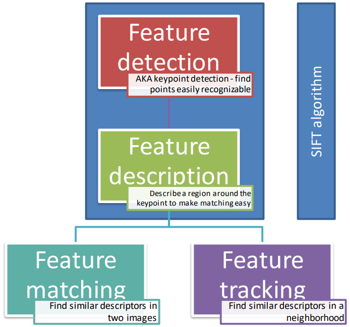

By using this algorithm, the image content gets mapped into local feature coordinates that are invariant to translation, rotation, scale and other transformations
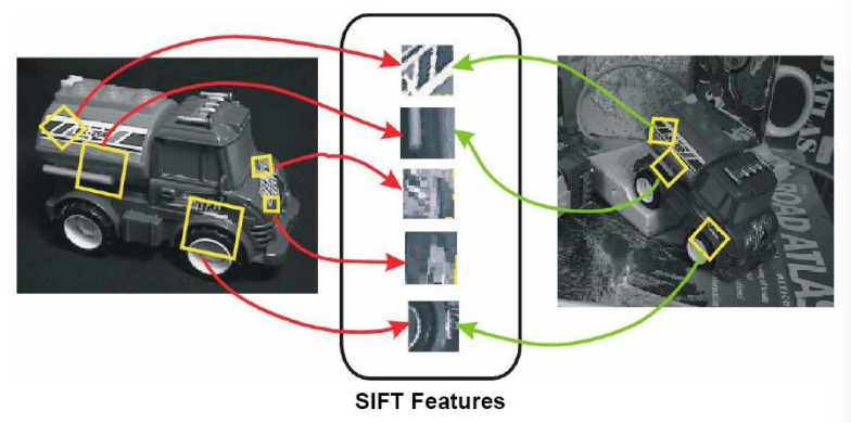
The SIFT features are:
- Local and robust to occlusions
- Distinctive between different objects in an image
- Dense, namely multiple features can be found even on small objects
- Efficient in the computation
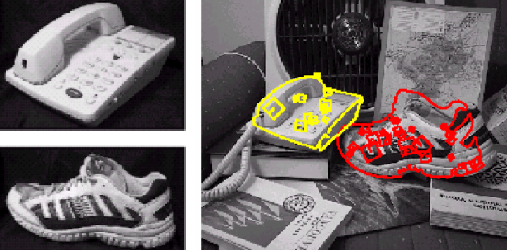
The steps of the algorithm are detailed as follows:
- Scale-space extrema detection
- Keypoint localization
- Orientation Measurement
- Descriptor calculation
Which we’ll analyse separately below.
Step 1: Scale-space extrema detection
SIFT uses the scale space organized in octaves to detect the main features, doubling the gaussian smoothing on every subsequent iteration (this in turn makes the smoothing effect constant on the down sampled images).
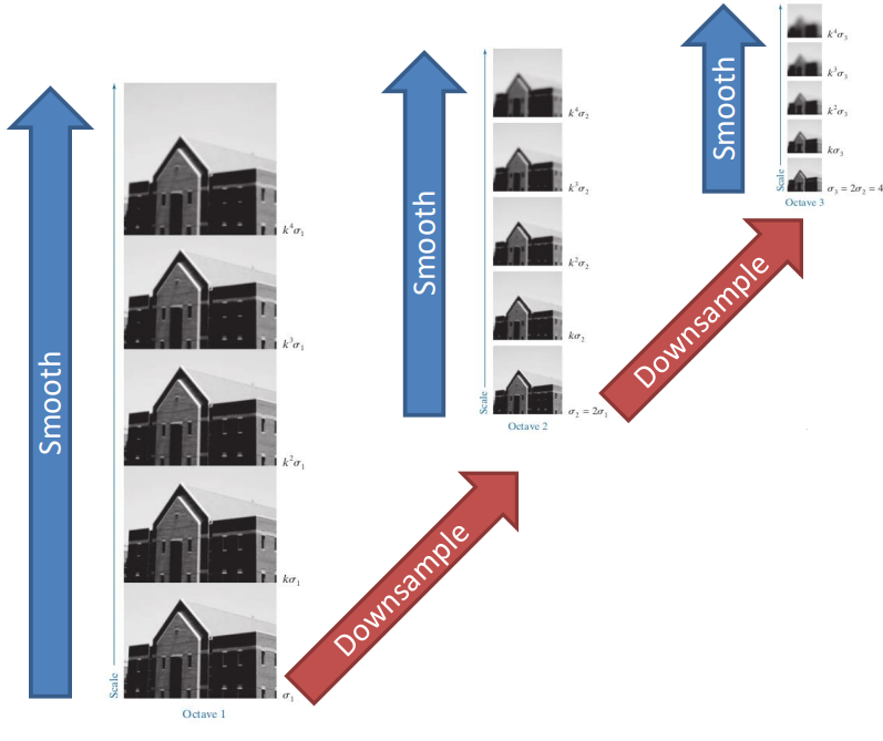
Within one octave, intermediate scaled are used, and the last image of each octave has the same amount of smoothing as the first image of the next octave. Each octave is composed of s intervals, which make s+1 images and the standard deviations are
\sigma, \, k\sigma, \, k^2\sigma, \, \dots, \, k^n\sigma
By merging together two octaves we get
\begin{aligned}
k\sigma&=2\sigma\\
k&=2^{1/s}
\end{aligned}
Different layers in the scale space are combined by subtracting consecutive layers. To do this, we need two additional images in the scale space to process the first and last image.

When the layer subtraction gets done, the resulting images are similar to the ones gotten for the edge detection algorithm, in which the higher octaves maintain only the more general details of the image
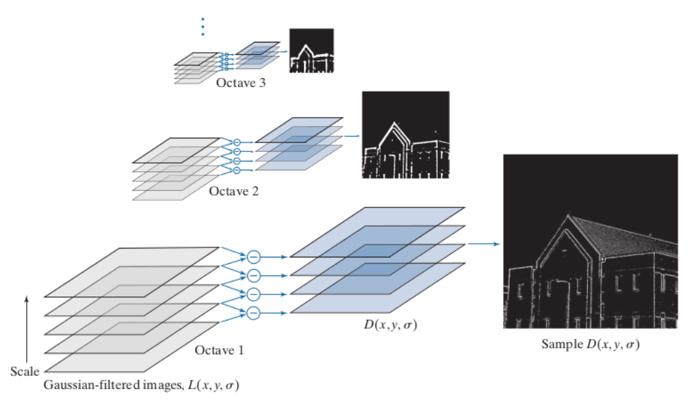
The subtraction of two layers is the difference between two smoothed image, such difference is called difference of gaussians (DoG) and is represented by the function
D(x, \, y, \, \sigma)
Because the algorithm applies the smoothing and the derivative filter we can combine them both into a single filter called the Laplacian of Gaussian (LoG). Such filter is obtained by using the gaussian filter
G(x, \, y) = \dfrac{1}{2\pi\sigma^2}\exp\left(-\dfrac{x^2+y^2}{2\sigma^2}\right)By considering the Laplacian \nabla^2 G(x, \, y) we can filter the image, which corresponds to filtering the image using G(x, \, y) and computing the Laplacian of the resulting image.
The smoothing step involves reducing the noise in the image, particularly at scales smaller than \sigma. This process aims to create a more uniform and even appearance across the image. Additionally, the technique identifies points of rapid change in brightness, known as zero-crossings, which often correspond to edges or boundaries in the image. The smoothing is isotropic, meaning it occurs uniformly in all directions, ensuring consistent results. To achieve effective noise reduction and edge detection, the filter size used for smoothing must be at least 6 pixels by 6 pixels.
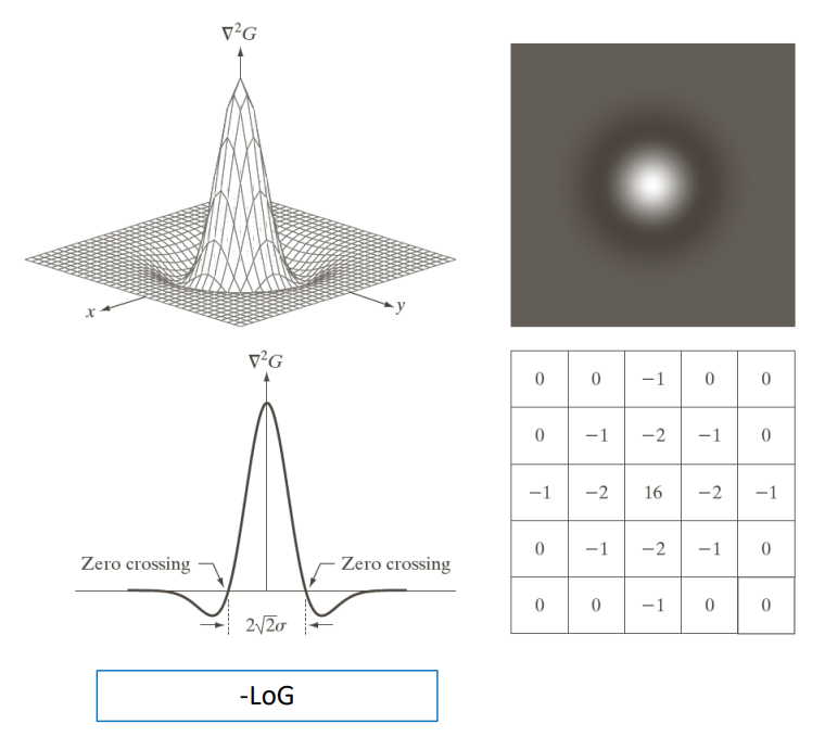
To approximate the DoG in the case of -\sigma_1>\sigma_2 we can use
D(x, \, y) = \dfrac{1}{2\pi\sigma_1^2} \exp\left(-\dfrac{x^2+y^2}{2\sigma_1^2}\right) - \dfrac{1}{2\pi\sigma_2^2} \exp\left(-\dfrac{x^2+y^2}{2\sigma_2^2}\right)Note: we have two different levels of smoothing, represented by \sigma_1 and \sigma_2. What this is saying is that \sigma_1 is bigger than \sigma_2, meaning that the first level of blurring is stronger or more spread out than the second one. It means we’re taking a less blurry image and subtracting from it a more blurry version. This helps highlight the edges and features in the image because the differences between the two versions are more pronounced.

Step 2: Keypoint localization
Keypoint localization within the SIFT algorithm focuses on determining the positions and scales of distinctive points, also known as keypoints, in an image. This process involves identifying significant locations where scale-space extrema are detected with high contrast and stability, ensuring that keypoints are accurately localized regardless of changes in scale, rotation, or illumination.
The technique compares the 8-neighbors in the current, previous and next scales obtained in the previous step.
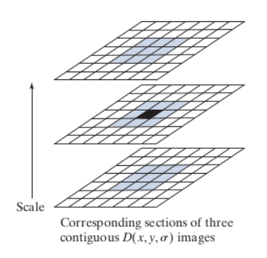
Note: sub pixel accuracy is obtained by interpolating the x, \, y and \sigma axis with Taylor expansions.
The Hessian matrix is computed for each pixel in the scale-space representation of the image. The Hessian matrix provides information about the local curvature or shape of the image intensity surface at that point. By analyzing the eigenvalues of the Hessian matrix, SIFT identifies regions where the intensity changes in multiple directions, indicating potential keypoints. Specifically, keypoints are localized at positions where the eigenvalues of the Hessian matrix satisfy certain criteria related to contrast, stability, and edge-like structures.
H=
\begin{bmatrix}
\dfrac{\partial^2 D}{\partial x^2} & \dfrac{\partial^2 D}{\partial x\partial y}\\[10pt]

\dfrac{\partial^2 D}{\partial y \partial x} & \dfrac{\partial^2 D}{\partial y^2}
\end{bmatrix}
=
\begin{bmatrix}
D_{xx} & D_{xy}\\
D_{yx} & D_{yy}
\end{bmatrix}
Using H we can discard point with a low gradient, for example
|D(\hat{x})| < 0.03And also discard edge points, which require both eigenvalues of H to be large.
Note: this process is similar to the one used to analyze Harris corners.
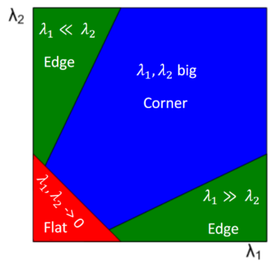
This selection process can also be done in the frequency domain, despite being more unstable.
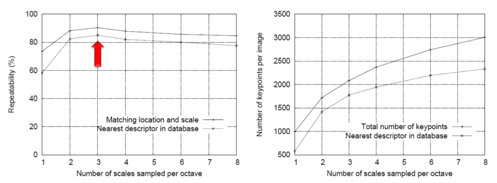
Note: the best value for s is 3.
The output of the keypoint localization is a set of keypoints with the associated scales.
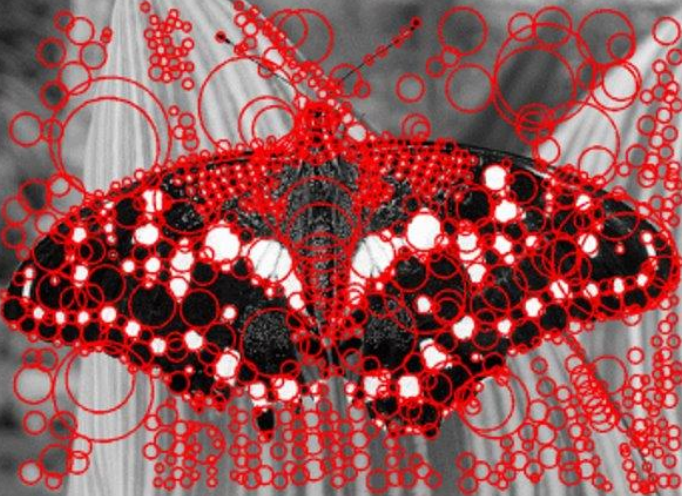
Step 3: Orientation measurement
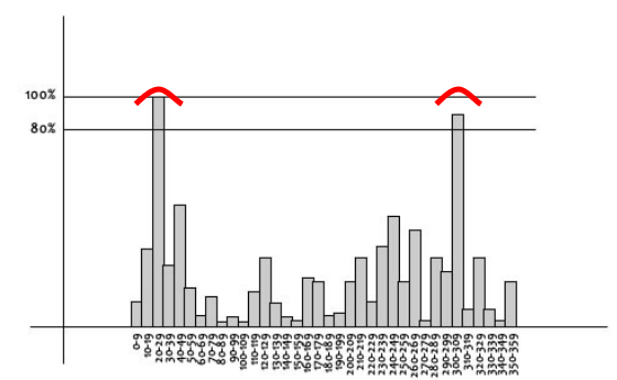
Orientation measurement involves determining the dominant orientation or direction of keypoint descriptors in an image. This step aims to enhance the robustness and invariance of keypoints by aligning them with the image gradient direction, allowing for consistent feature matching across different orientations. SIFT computes the gradient magnitude and orientation for each pixel in the keypoint’s local neighborhood and then constructs a histogram of gradient orientations. The peak in this histogram indicates the dominant orientation, which is used to rotate the descriptor accordingly, making it invariant to image rotation.
The gradient magnitude is computed as
M(x, \, y) = \sqrt{(L(x+1, \, y)-L(x-1, \, y))^2+(L(x, \, y+1)-L(x, \, y-1))^2}While the orientation angle is
\theta(x, \, y) = \tan^{-1}\left(\dfrac{L(x, \, y+1) - L(x, \, y-1)}{L(x+1, \, y)-L(x-1,\,y)}\right)The built histogram is made out of 36 bins of 10° each

The peak of the histogram is highlighted, and now we need to fit a parabola to the 3 bins close to the peak to refine its location.
Secondary peaks are also considered by considering the ones that are at least 80% of the height of the highest peak. A new keypoint is created with the orientation set to the secondary peak.
The following image represents an example of the keypoint detection.
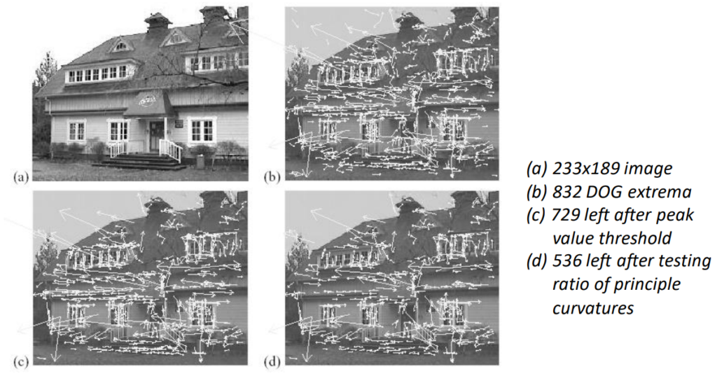
Step 4: Descriptor calculation
Descriptor calculation involves creating compact representations of the local image structure around keypoints. These descriptors capture unique patterns of gradient directions and magnitudes within a keypoint’s neighborhood, making them highly distinctive and able to withstand transformations like rotation. This allows for accurate matching of keypoints across different images.
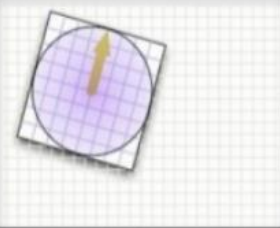
To compute the descriptor, gradients are calculated in terms of magnitude and direction within a 16\times 16 neighborhood around each keypoint. These gradient values are then weighted using a Gaussian function centered on the keypoint.
This 16\times 16 neighborhood is divided into 4\times 4 pixel regions, and a histogram is created for each region. Each histogram has 8 bins, with each bin representing a 45° range of gradient directions.
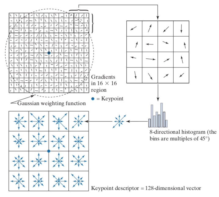
The descriptor size refers to the number of elements representing each keypoint. In this case, the descriptor has 128 elements. These elements are derived from dividing the keypoint’s local neighborhood into 16 regions, each with a histogram of 8 values. Each element in the descriptor vector is usually stored as a single byte, creating a compact representation of the keypoint’s visual features.
Additional details are taken into account to improve its performance in various conditions. Firstly, to enhance invariance to illumination changes, the feature vectors are normalized to have a unit length. This normalization helps ensure that the descriptors are not affected by varying lighting conditions, making the algorithm more reliable across different environments. Secondly, to bolster robustness against large gradient magnitudes, a threshold of 0.2 is applied to all components of the feature vector. This thresholding helps mitigate the effects of nonlinear illumination variations, such as camera saturation. Additionally, after thresholding, further normalization is conducted to ensure that the feature vectors are scaled to a consistent magnitude, enhancing the algorithm’s consistency and accuracy in feature matching and recognition tasks.
Examples:
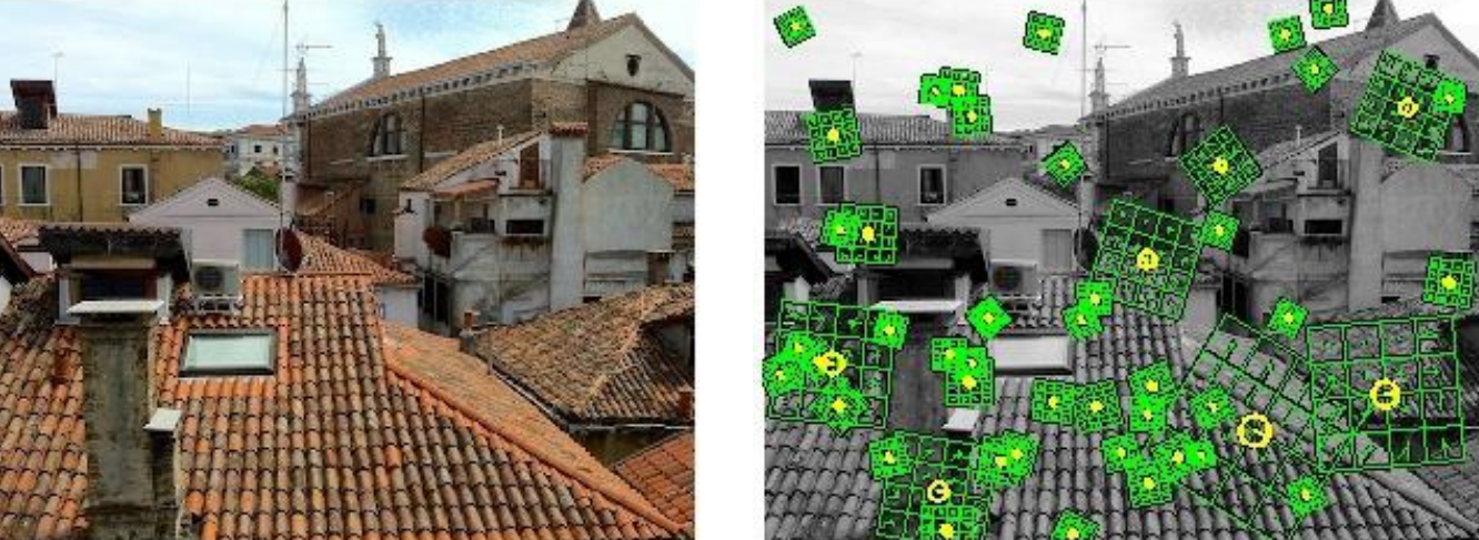
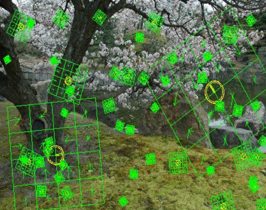
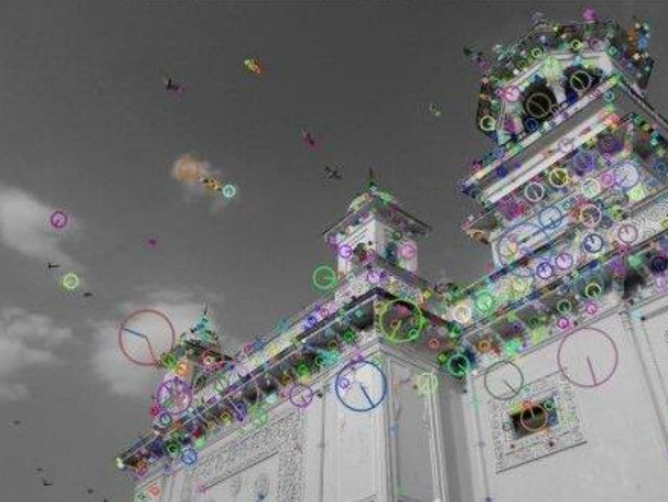
Scale / Illumination / Orientation invariances
- Scale Invariance: SIFT is invariant to scale because it detects features at multiple scales within an image. By constructing a scale-space pyramid and identifying key points across different levels of blurring or smoothing, SIFT ensures that key features are detected regardless of their size in the original image. This allows SIFT to handle objects or scenes that appear at different scales within an image or across different images.
- Illumination Invariance: SIFT achieves invariance to illumination changes by normalizing the feature vectors to have a unit length. This normalization ensures that the descriptors are unaffected by variations in lighting conditions across different images. Additionally, SIFT applies thresholding to mitigate the effects of nonlinear illumination changes, such as camera saturation. These techniques help maintain the discriminative power of the descriptors, making them robust to changes in illumination.
- Orientation Invariance: SIFT is invariant to orientation by determining the dominant orientation of keypoints and rotating the local image patches accordingly during descriptor calculation. By aligning the descriptors with the dominant orientation of keypoints, SIFT ensures that features are consistently represented regardless of their orientation in the image. This allows SIFT to accurately match keypoints across images with different orientations, enabling robust feature matching and recognition.
Beyond SIFT
There are several methods that go beyond SIFT, namely
- PCA-SIFT
- SURF
- GLOH
PCA-SIFT
Principal Component Analysis (PCA) SIFT, or PCA-SIFT, is a variant of the popular Scale-Invariant Feature Transform (SIFT) algorithm. PCA-SIFT integrates the principles of PCA, a dimensionality reduction technique, with the SIFT algorithm to enhance its efficiency and computational speed. The data gets projected onto a lower dimension linear space that minimizes the mean square distance between original data points and their projection.
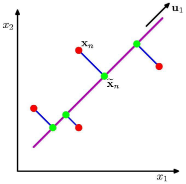
By applying PCA to the high-dimensional feature space generated by SIFT, PCA-SIFT reduces the dimensionality of feature descriptors while preserving their discriminative power. This reduction is based on the eigenvalue decomposition of the covariance matrix. The largest eigenvectors capture the most important information. By using them as a basis, we can represent the data more efficiently and effectively, focusing on the key features that contribute the most to its overall structure.
This reduction in dimensionality not only accelerates the matching process but also improves the algorithm’s robustness to variations in scale, rotation, and illumination.
For example
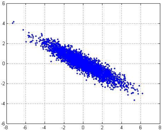
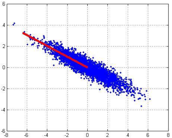
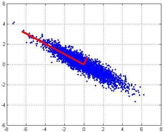
In this algorithm, steps 1 to 3 are the same as in SIFT, but the descriptor calculation is different. Instead of using SIFT’s method, this algorithm looks at a 41\times 41 patch around each keypoint, normalized to a standard direction.
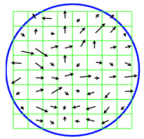
In SIFT, feature descriptors are created using weighted histograms of gradient orientations within local image areas. PCA-SIFT uses a different method: it combines horizontal and vertical gradients into a long vector and normalizes this vector to have a unit norm, ensuring that the scale is consistent across different feature vectors.
PCA is then used to reduce the dimensionality of this feature vector.
SURF
Speeded Up Robust Features (SURF) offers accelerated computation while maintaining robustness to variations in scale, rotation, and illumination. By employing integral images and fast Hessian matrix approximations, SURF achieves remarkable speed improvements compared to SIFT, making it particularly suitable for real-time applications and large-scale image processing tasks.
Note: compared to SIFT, SURF is less robust to illumination and viewpoint changes.
An integral image I_{\Sigma}(x, \, y) is an image in which each pixel represents the sum of all pixels in the rectangle between (0, \, 0) and that pixel. For pixel i we get
I_{\Sigma}(x_i, \, y_i) = \sum_{i=0}^{x_i-1} \sum_{j=0}^{y_i -1} I(i, \, j)For example, by considering the image below
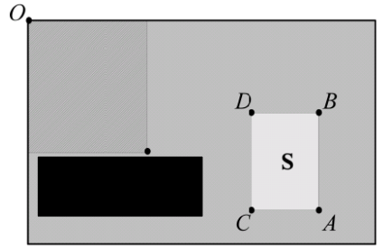
We get
S=A+D-B-C
Box filters are essential in computing SURF by enabling the efficient calculation of integral images. Box filters apply uniform weights to all pixels within a rectangular area, allowing for quick computation of integral images when convolved with the input image.
A box filter consists of black and white rectangles, where white represents a positive weight and black represents a negative weight. These filters help approximate the partial derivatives in the Hessian matrix.

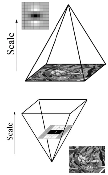
While the standard SIFT algorithm involves two steps of Gaussian smoothing and subsampling, SURF achieves a similar effect by using filters of increasing size to build the scale space. This approach simplifies and speeds up the computation process.
Regarding the orientation instead, we can consider a neighborhood of size 6\sigma and evaluate the gradients in the x and y directions using the Haar wavelets.
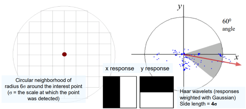
Haar wavelets are a type of wavelet function used characterized by their simple, step-like shape, consisting of a positive portion followed by an equal negative portion. Haar wavelets are particularly effective in representing abrupt changes or discontinuities in images.
By plotting such responses in a 2-dimensional space and summing up horizontal and vertical responses we can determine the final orientation of the feature. The quantization of the responses is in bins of 60°.
We divide the image into 16 regions. For each of these regions, we calculate the sum of the responses in both the horizontal (dx) and vertical (dy) directions, as well as the sum of their absolute values (modules). Then, we normalize these values to make them comparable. Each region contributes 4 elements to the feature vector, resulting in a total of 64 elements for the entire image. This feature vector encapsulates important information about the local image structure, helping to identify distinctive features that are robust to changes in scale, rotation, and illumination.
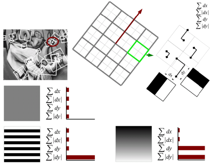
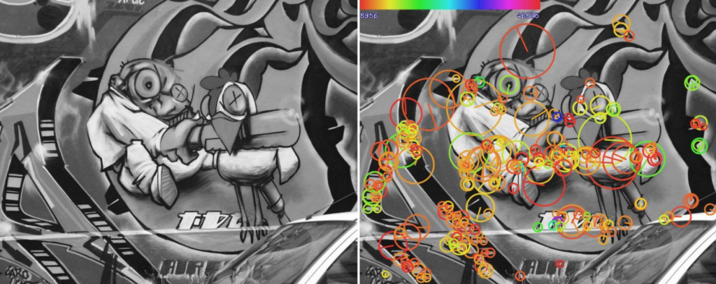
And example of the SURF feature extraction
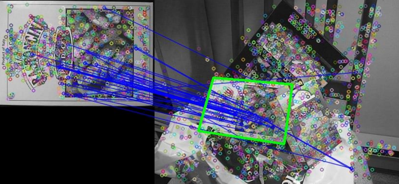
And SURF matching
GLOH
Gradient Location-Orientation Histogram is obtained by modifying the fourth step of the SIFT algorithm, specifically, with GLOH, the descriptors are computed using polar coordinates.
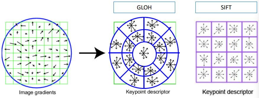
We divide the keypoint’s surrounding area into three concentric circles or “bins” with radii of 6, 11, and 15 pixels. Within each bin, we further divide it into 8 angular sections. This creates a total of 24 bins (1 central + 8 in the inner circle + 8 in the outer circle) for each of the 16 possible orientations, giving us a total of 272 orientation bins. To reduce the complexity of these bins, PCA is used to condense them into a more manageable 128-dimensional feature vector. This process retains the most important information while significantly reducing the computational load and memory requirements for feature matching and recognition tasks.
Other approaches
There are also other approaches to feature detection that are completely not based on SIFT.

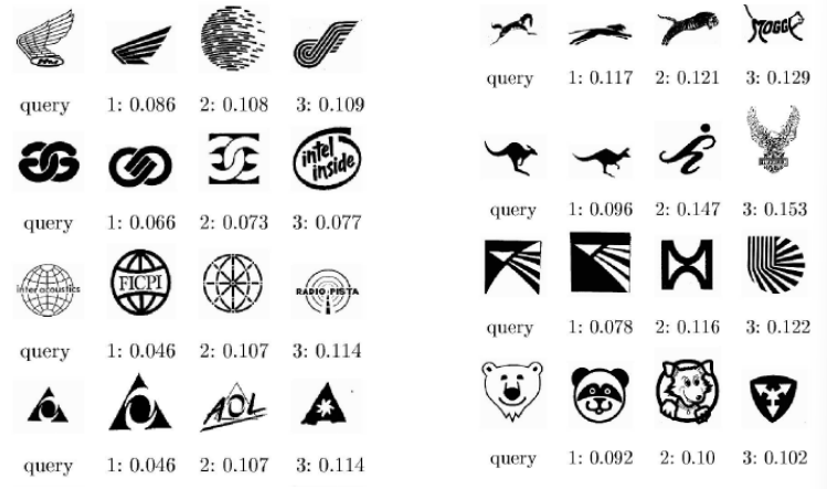
- The Shape Context algorithm is particularly effective for detecting and recognizing objects even when they’re undergoing changes in scale, rotation, or deformation. It works in the following way:
- Shape Descriptor Creation: Initially, the algorithm represents the shape of an object using a set of points called “landmark points”. These points are usually extracted from the object’s edges.
- Shape Context Calculation: For each landmark point, the algorithm computes a descriptor called the “shape context”. This descriptor captures the spatial distribution of other landmark points around it. It quantifies the relative positions of these points in terms of distance and angle. Polar coordinates are used.
- Histogram Creation: The shape contexts are then organized into histograms. Each landmark point’s histogram represents the distribution of other points around it in terms of distance and angle. The histogram bins encode information about the local shape structure.
- Comparison and Matching: To compare two shapes, their respective histograms are compared using distance metrics such as the Earth Mover’s Distance (EMD) or Chi-Squared distance. This comparison evaluates the similarity between the shapes based on their local structure.
- Object Recognition and Matching: The Shape Context algorithm enables object recognition and matching by finding correspondences between the histograms of different shapes. By identifying similar histograms, the algorithm can detect objects in images, even if they’re undergoing transformations like scaling, rotation, or deformation.
Example video matching:
Example shape matching:
- Local binary pattern (LBP) operates by examining the relationship between a central pixel and its neighboring pixels within a local region. The algorithm works as follows:
- Image Partitioning: The image is divided into small, non-overlapping regions called cells or patches.
- Feature Extraction for Each Cell: For each pixel in the cell, compare its intensity value with the intensity values of its neighboring pixels. Based on the comparisons, assign a binary value (0 or 1) to each neighbor pixel, indicating whether its intensity value is greater than or equal to that of the central pixel.
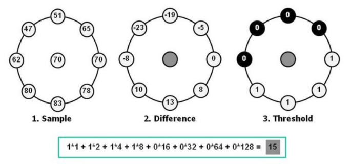
For example, we can distinguish the following patterns:

- Continue LBP
- Encoding the Pattern: Concatenate these binary values in a clockwise or counterclockwise order to form a binary number. This binary number represents the pattern of intensity variations in the local neighborhood of the central pixel.
- Histogram Calculation: After encoding patterns for all pixels in the cell, a histogram of the occurrences of different binary patterns is computed. The histogram bins represent the possible patterns, and the histogram values represent how often each pattern occurs within the cell.
- Feature Vector Formation: Combine histograms from all cells to form a feature vector representing the texture of the entire image.

- BRIEF descriptor works in the following way:
- Selection of Pairs of Pixels: BRIEF operates by comparing pairs of pixels in an image. These pairs are chosen randomly from a predefined distribution. Usually, Gaussian distribution is used to sample pairs around the center pixel. Other distributions are shown in the picture below
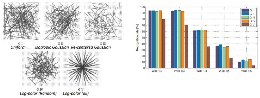
- BRIEF descriptor continue:
- Intensity Comparison: For each pair of pixels selected, a simple intensity comparison is made. If the intensity value of the first pixel is greater than that of the second pixel, the result for that pair is 1; otherwise, it’s 0.
- Descriptor Creation: After performing intensity comparisons for all pairs, a binary string is formed based on the results. This binary string serves as the BRIEF descriptor for the particular keypoint or patch of the image.
- Matching: During matching or recognition tasks, BRIEF descriptors of keypoints or patches in different images are compared using the Hamming distance. The hamming distances for matching pair of points are shown in blue, while non-matching pairs are shown in red.

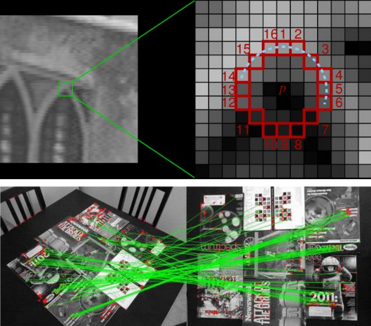
- Oriented FAST and Rotated BRIEF (ORB) is an enhancement of the original BRIEF algorithm, designed to provide rotation invariance to keypoint descriptors. It combines the efficiency of the FAST corner detector with the binary descriptors of BRIEF, while also introducing orientation assignment to handle rotation.
